XLOOKUP Excel With Examples: Complete Guide

The XLOOKUP function in Excel is a powerful and flexible tool designed to replace older lookup functions like VLOOKUP and HLOOKUP. Unlike these traditional functions, XLOOKUP can search both vertically and horizontally, making it ideal for retrieving specific values from any range in a table. With added benefits like default exact matching and the ability to handle errors more gracefully, XLOOKUP makes data retrieval in Excel easier and more reliable.

In this article, we will cover how XLOOKUP works, its syntax, and practical examples to help you make the most of this versatile function.

XLOOKUP Function in Excel With Examples

What is XLOOKUP in Excel

XLOOKUP is a powerful function in Excel designed to search for a specific value in a range and return a corresponding value from another range. It replaces older functions like VLOOKUP and HLOOKUP, addressing their limitations by allowing for more flexible searches, including reverse lookups and partial matches.

XLOOKUP Formula in Excel with Example

=XLOOKUP(lookup_value, lookup_array, return_array,  [if _not_found], [match_mode], [search_mode])

XLOOKUP Formula Explanation

=XLOOKUP(search for this value, in this range, and Return a match from this range).

Arguments Explained

• lookup_value: The value you want to search for.
• lookup_array: The range of cells where Excel will search for the lookup value.
• return_array: The range of cells from which to return the result.
• if_not_found (optional): Value to return if no match is found.
• match_mode (optional): Specifies the type of match (exact, approximate, or wildcard).
• search_mode (optional): Determines the search direction (first-to-last or last-to-first).

• search_mode (Optional): where we can specify how the function should look up the value.

How to Enable XLOOKUP in Excel

To access the XLOOKUP function in Excel, you need to be using a version of Excel that supports it.

How to Enable XLOOKUP in Excel 365

XLOOKUP is included in Excel 365, which is a subscription-based version of Excel that receives regular updates and new features.

How to Enable XLOOKUP in Excel 2019

XLOOKUP was introduced in Excel 2019, which is a one-time purchase version of Excel. However, it might not be available in older versions of Excel, such as Excel 2016 or earlier.

Step-by-Step Guide to Using XLOOKUP in Excel

Step 1: Open Excel

Start by opening your Excel application and loading the worksheet containing your data.

Step 2: Select a Cell

Click on an empty cell where you want to display the result of your XLOOKUP function.

Step 3: Start Typing the Formula:

• Type =XLOOKUP( into the selected cell. Excel will prompt you with a list of arguments.

Step 4: Enter Required Arguments:

• lookup_value: Specify the value you are searching for (e.g., a cell reference like A2).
• lookup_array: Select the range where Excel should look for this value (e.g., B2:B10).
• return_array: Choose the range from which you want to retrieve data corresponding to the found value (e.g., C2:C10).

Example formula:

=XLOOKUP(A2, B2:B10, C2:C10)

Optional Arguments:

• If desired, add optional arguments such as if_not_found to handle cases where no match is found.
• Use match_mode to specify how closely you want Excel to match your lookup value (0 for exact match, 1 for next largest, etc.).
• Set search_mode if you want to control whether it searches from first to last or vice versa.

Step 5: Complete the Formula

Close the parentheses and press Enter. Your formula should now return the corresponding value based on your criteria.

XLOOKUP Example in Excel: 6 Examples Explained

Below are some examples through which the XLOOKUP function will be easily understandable.

Example 1: Using XLOOKUP for Exact Matches

This function in XLOOKUP is by default. Follow the below steps to Lookup a value:

Step 1: Format your data

Enter you Data

Now, if we want to get the math marks of Carry then follow the next step

Step 2: Enter the Formula

We will enter =XLOOKUP(E2, A2:A5, B2:B5) in the F2 cell to get the marks of carrying.

Enter the Formula

Then we will get the math marks for carry.

Example 2: How to Approximate Match in Excel

If you want to find the closest (approximate) match to a specified value, use match mode -1 (next smaller) or 1 (next larger):

Step 1: Format your data

Step 2: Enter Formula

Let’s consider the below example for Approximate match mode.

Format your Data

Formula used is : =XLOOKUP(lookup value, in this range, Return a value from this range, -1)

Here -1 will return the approximate value which is smaller than the lookup value. 

Note: The user can also use 1 instead of -1 to return a value larger than the lookup value. The XLOOKUP function can also work for Unsorted data.

Example 3: How to Use Left Lookup in Excel

Unlike VLOOKUP, XLOOKUP can perform a left lookup, allowing you to search for values on the left side of the data:

Step 1: Format your data

Step 2: Use Formula

Using INDEX and MATCH in Excel left lookup can be performed but to make it simple and quick you can also use the XLOOKUP function. This XLOOKUP function is used to search the values which are on the left side of the searched values.

The formula used: = XLOOKUP(Search for this value, from this range, and return the output from this range)

Here the output we are looking for will be from the left side of the column.

Example 4: How to Use XLOOKUP on Multiple Values

You can combine XLOOKUP with additional functions for more complex lookups. To retrieve a value based on multiple conditions, use concatenation or an array formula:

Step 1: Format your data

Enter and Format your Data

Now, if we want to get the Math and English marks for carrying then follow the next step

Step 2: Enter the Formula

We will enter =XLOOKUP(E2,A2:A5,B2:C5) in F2 cell.

Enter the Formula

Step 3: Marks Obtained

Then we will get the Math and English marks.

Marks Obtained

Example 5: How to Use Nested XLOOKUP function in Excel

Follow the below steps to use nested XLOOKUP functions:

Step 1: Format your data

Format your Data

Now, if we want to get the math marks of Carry by two-way lookup then follow the next step.

Step 2:Enter the Formula

We will enter =XLOOKUP(F1,B1:C1,XLOOKUP(E2,A2:A5,B2:C5)) in F2 cell.

Here, XLOOKUP(E2, A2:A5, B2:C5) is{100,80} which is an array mark of Carry. In the outer XLOOKUP formula, we are looking for the subject name which is in the F1 cell and the lookup array is B1:C1.

Enter the Formula

Step 3: Marks Displayed

Then we will get the math marks of carry.

Marks Displayed

Example 6: How to Use Not Found in Excel

Follow the below steps when the LOOKUP function returns the Not Found message:

Step 1: Format your data

Format your Data

If we want the marks of Sunny who is not in the dataset

Step 2: Enter Formula

We will enter =XLOOKUP(E2,A2:A5,B2:B5,”Not Found”) in F2 cell.

Enter your Data

Step 3: Not Found Displayed

Then it will show Not Found.

Not Found Displayed

Example 4: How to Use SUM function in Excel

Follow the below steps to find the sum of a range:

Step 1: Format your data.

Format your Data

If we want the total math marks from Harry to Jonny then do the next step

Step 2: Enter Formula

We will enter =SUM(XLOOKUP(E2,A2:A5,B1:B6):XLOOKUP(F2,A2:A5,B1:B6)) in G2 cell this simply means =SUM($B$2:$B$5).

Enter your Formula

Step 3: Sum Displayed

Then we will get the sum.

Sum Displayed

Example 5: How to Use Horizontal Lookup in Excel

Step 1: Format your data

Format your Data

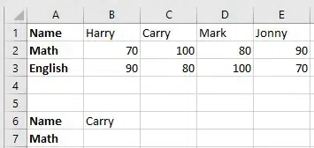
Now, if we want to get the math marks of Carry then follow the next step

Step 2: Enter the Formula

We will enter =XLOOKUP(B6,B1:E1,B2:E2) in B7 cell.

Format your Data

Step 3: Carry Marks Displayed

Then we will get the math marks of Carry

Carry Marks Obtained

Example 6: How to Use Last Match in Excel

Follow the below steps to use last match in Excel:

Step 1: Enter your data

Step 2: Enter the XLOOKUP Formula

By default, the XLOOKUP Function performs a top-to-bottom search. But if the user wants to change this order and search for the bottom to top then the formula should be: =XLOOKUP(Search for the value, in this range, return the output from this range, -1)

Note: -1 in this formula should be the 6th parameter) 

XLOOKUP Vs VLOOKUP: Key Differences

XLOOKUP and VLOOKUP are Excel functions used for finding information in a table, but they have differences:

Note: XLOOKUP is more versatile and user-friendly, especially for complex datasets and lookups across multiple columns or rows.

Advanced XLOOKUP Techniques

• Nested XLOOKUP: Use XLOOKUP within another XLOOKUP for two-way lookups.
• Horizontal Lookups: Perform searches across rows instead of columns.
• Using XLOOKUP for Summation: Calculate totals over a specified range using XLOOKUP with SUM.

Conclusion

In conclusion, XLOOKUP is a revolutionary addition to Excel that addresses the limitations of VLOOKUP and HLOOKUP. By mastering XLOOKUP, you can perform efficient data searches, streamline your workflow, and enhance your overall productivity. Whether you’re a financial analyst, data scientist, or small business owner, leveraging XLOOKUP in your daily tasks will save you valuable time and effort.