Excel VLOOKUP Function - Excel Guide for Beginners
Last Updated :
02 Jul, 2025
How to do VLOOKUP in Excel - Quick Steps
- Prepare Your Data
- Enter the VLOOKUP Formula >> Press Enter
- Use a Cell Reference for Flexibility
- Copy the Formula for Multiple Rows
Adding clickable links to your document is a simple yet powerful way to connect readers to external websites, email addresses, or even other sections within the same file. Knowing how to add a hyperlink in MS Word allows you to enhance your content and improve navigation for your audience. Whether you're creating a report, a resume, or a reference document, inserting hyperlinks ensures a more interactive and user-friendly experience. In this guide, you’ll learn the quick steps to insert a hyperlink in Microsoft Word, edit existing links, and format them to match the style of your document.
What is the VLOOKUP Function in Excel
The term VLOOKUP stands for Vertical Lookup. It is designed to search for a specific value in the first column of a table (lookup column) and retrieve corresponding data from a different column in the same row.
Syntax of VLOOKUP Formula
VLOOKUP(lookup_value, table_array, col_index_num, [range_lookup])
Arguments:
1. lookup_value: The value you want to search for (e.g., a specific ID, name, or product code).
2. table_array: The range of cells that contains the data (the table you're searching through).
3. col_index_num: The column number (from the table array) that contains the data you want to retrieve. The first column is 1, the second is 2, and so on.
4. [range_lookup] (optional): If TRUE (or omitted), it searches for an approximate match. If FALSE, it searches for an exact match.
TRUE indicates an approximate match, and it's the default value if this argument is omitted.FALSE indicates an exact match.
Note: If nothing is specified by the user, by default this value is set to be 'True' and it searches for an approximate match. This argument is completely optional.
How VLOOKUP Works
VLOOKUP operates by scanning the first column of a table vertically until it finds a match for the lookup value. Once it finds this match, it returns a value from the same row, but from another column, which is specified by the user. This makes it particularly useful for pulling associated information, like retrieving a price from a product ID or a name from an employee ID.
How to Use Excel VLOOKUP Function with Example (For Beginners)
Managing inventory can be tough, especially when you need to quickly find product prices during sales. Instead of manually searching through long lists, Excel's VLOOKUP function makes it easy. Simply input a product ID, and VLOOKUP retrieves the matching price or related details instantly, saving you time and reducing errors.
Step 1: Prepare Your Data
Make sure your data is arranged with the lookup column (the column you will search) as the first column of your table. For example, if you’re looking up product prices by ID, the IDs should be in the first column:
- List all product IDs in the first column (A).
- Product Name in second column (B).
- Ensure the corresponding prices are in a column to the right of the IDs and Product Name, here we have mentioned that in column (C).
 Prepare your Data
Why Proper Organization Matters:
Having the lookup column as the first column ensures VLOOKUP works correctly. Incorrect table organization can lead to errors or incorrect results.
Select a cell where you want the price to appear when you type a product ID.
- Select a Cell for the Result: Click in the cell where you want the VLOOKUP result to appear, here we have selected D2.
- Start the Formula: Type
=VLOOKUP( in cell D2.
 Enter the VLOOKUP Formula
Step 3: Define the Lookup Value
Enter the value you want to search for in the formula:
- Use a cell reference, like
A2, or type a value directly in quotes, such as "001". - Example: If searching for a product ID in cell D2, start the formula as:
=VLOOKUP(A2, or =VLOOKUP("001", - Add a comma after the lookup value to move to the next part of the formula.
 Define the Lookup Value
Step 4: Specify the Table Array
- Select the data range where you want to search, e.g.,
A1:C4 (IDs in column A and Prices in column C). - Highlight the range by clicking and dragging.
- Add a comma after selecting the table array.
 Specify the Table Array
Step 5: Indicate the Column Index Number
- Enter the column number from which you want to retrieve the data.
- For example, if prices are in the third column (C), type 3 in the formula:
=VLOOKUP(D2, A1:C4, 3,. - Add a comma after the column number.
Purpose of col_index_num: The col_index_num in a VLOOKUP formula specifies which column in the table_array to pull the data from, once a match is found for the lookup_value in the first column of that array.
Why Use 3?
In the range A1:C4:
- Column A has Product IDs.
- Column B has Product Names.
- Column C has Prices.
The number 3 tells Excel to return data from the third column (Prices).
This instructs Excel to look within the range A1 to C4 and return the value from the third column of the range when it finds a match.
 Indicate the Column Index Number
Step 6: Choose the Range Lookup Type
- Decide if you need an exact match or an approximate match for your search.
- For exact matches (e.g., finding the exact price for a product ID), type FALSE in the formula.
- Add a closing parenthesis
) to complete the formula.
Purpose of range_lookup:
- FALSE: Ensures VLOOKUP finds an exact match for the lookup value.
- TRUE: Allows approximate matches, typically used when the data is sorted.
Why Use FALSE?
Using FALSE ensures VLOOKUP only returns a value if the exact Product ID exists in the first column (e.g., column A).
- If no match is found, it shows
#N/A, preventing incorrect results. - This is important for precise searches, like finding exact prices or IDs.
By setting the parameter to FALSE, your formula ensures accuracy and avoids errors caused by approximate matches.
This ensures that the exact Product ID entered in cell D2 is matched in column A, and the corresponding price from column C is returned. If no exact match is found, the function will display an #N/A error, indicating the ID is not in the list. This is safer than returning an incorrect or approximate price.
 Choose the Range Lookup Type
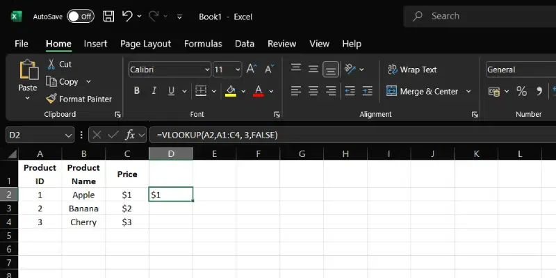
- Press Enter: Your complete formula in cell D2 should look like this:
=VLOOKUP(A2, A1:C4, 3, FALSE)
- View the Result: After pressing Enter, cell D2 should display
$1, which is the price of the product with ID 001.
 Complete and Execute the Formula
How to VLOOKUP between two Excel Spreadsheets
Using the VLOOKUP function to connect data between two Excel sheets within the same workbook is a powerful way to improve efficiency and smooth your workflow. Here’s an easy step-by-step guide to help you use VLOOKUP across two sheets.
Example:
Imagine you have an Excel workbook with two sheets.
Sheet1 ("Employee Info") contains a list of employee IDs and their names.
| Employee ID | Employee Name |
|---|
| 101 | John Doe |
| 102 | Jane Smith |
| 103 | Emily White |
Sheet2 ("Contact Details") contains a list of employee IDs and their corresponding email addresses.
Goal:
Use VLOOKUP to display employee email addresses in Sheet1 based on their IDs.
Step 1: Set Up VLOOKUP in Sheet1
Navigate to Sheet1 ("Employee Info") and click on cell C2 (right next to the first Employee ID).
 Set Up VLOOKUP in Sheet1
Type in the following formula in cell C2 of Sheet1:
=VLOOKUP(A2, Sheet2!A:B, 2, FALSE)
Here’s a simple explanation of each part of the formula:
- A2: Refers to the cell in Sheet1 containing the Employee ID you want to look up.
- Sheet2!A:B: Tells Excel to search in columns A to B of Sheet2. The "Sheet2!" notation indicates the data is on another sheet.
- 2: Specifies that the result you want (the email address) is in the second column of the range in Sheet2.
- FALSE: Ensures the formula returns an exact match for the Employee ID.
 Enter the VLOOKUP Formula
- Press Enter: After typing the formula in cell C2, press Enter. The result, "[email protected]" will appear for Employee ID 101.
- Copy the Formula: Click on cell C2.
- Drag the Fill Handle: Use the small square at the bottom-right corner of the cell. Drag it down to copy the formula to the other cells in Column C.
- Auto-Adjust: Excel will automatically adjust the formula for each row, showing the corresponding email addresses for the other Employee IDs (C3, C4, etc.).
 Execute and Extend the Formula
Step 4: Verify the Results
Check that the correct email addresses appear next to the corresponding employee names in Sheet1. The complete "Employee Info" table should now look like this:
Troubleshooting
- If you get an
#N/A error, check to ensure that the Employee IDs match exactly between Sheet1 and Sheet2. Verify that there are no extra spaces or different formats (e.g., numbers stored as text). - Ensure that the VLOOKUP range includes all rows in Sheet2 if new data is added later.
How to VLOOKUP between two Workbooks
VLOOKUP is a powerful tool that can pull data from one workbook to another, making it easy to consolidate and analyze information stored in separate files. Here’s a step-by-step guide on how to use VLOOKUP across two Excel workbooks.
Example:
Suppose you're working with sales data and you have two Excel workbooks:
Workbook1 ("Sales Data.xlsx") contains sales transaction details including Transaction IDs and the amounts.
 Prepare your Data in Sheet1
Workbook2 ("Employee Sales.xlsx") contains Transaction IDs and the corresponding employee names who made the sales.
 Prepare your Data in Sheet2
Goal
You want to add a third column to the "Sales Data.xlsx" workbook that displays each employee's name associated with the transactions by linking the data using the Transaction ID.
Step 1: Open Both Workbooks
- Open "Sales Data.xlsx" (Workbook1) and "Employee Sales.xlsx" (Workbook2) simultaneously.
- This ensures Excel can reference the second workbook while creating the VLOOKUP formula.
Step 2: Set Up VLOOKUP in Workbook1
- Go to Workbook1 ("Sales Data.xlsx").
- Select cell C2 (next to the first Transaction ID).
 Set Up VLOOKUP in Workbook1
Type in the following formula in cell C2 of "Sales Data.xlsx":
=VLOOKUP(A2, '[Employee Sales.xlsx]Sheet1'!$A$1:$B$3, 2, FALSE)
Here's what each part of the formula does:
- A2: The cell contains the first Transaction ID in "Sales Data.xlsx" that you are using as the lookup value.
- '[Employee Sales.xlsx]Sheet1'!$A$1:$B$3: Specifies the range in "Employee Sales.xlsx" where the VLOOKUP should search for the Transaction ID. Ensure that the range includes all necessary rows and columns, and it’s important to use absolute references (with
$) so the range does not shift when the formula is copied. - 2: Indicates that the value you want to return (the employee name) is in the second column of the specified range.
- FALSE: Specifies that you need an exact match for the Transaction ID.
 Enter the VLOOKUP Formula in Sales Data Workbook
Press Enter to execute the formula in cell C2. If correctly entered, cell C2 will now display "John Doe", corresponding to Transaction ID T001.
To apply the same formula to the other transactions:
- Click on cell C2.
- Drag the fill handle down through the column to fill the rest of the cells in Column C with the VLOOKUP formula, adjusting it for the subsequent rows (C3, C4, etc.).
 Execute and Extend the Formula
Step 5: Verify the Results
Check that the correct employee names appear next to the corresponding transaction IDs in "Sales Data.xlsx". The complete table should look like this:
Troubleshooting
- If you get an
#N/A error, ensure that the Transaction IDs match exactly between the two workbooks. Also, verify that both workbooks are open while using VLOOKUP. - If Workbook2 is closed, Excel may not be able to retrieve the data. In some cases, Excel can store and display the cached result, but it’s best to have both files open during setup.
Common Troubleshooting Tips for VLOOKUP Function in Excel
Sometimes you may find that VLOOKUP not working, so in the below examples, you can find why your VLOOKUP Function not working and how to fix the error.
1. Handling #N/A Errors
- Issue: The #N/A error is commonly returned when VLOOKUP cannot find a match.
- Fix: Ensure that the
lookup_value actually exists in the first column of your table_array. Double-check for any typing errors or mismatched data types (e.g., numbers stored as text).
2. Correcting #VALUE! Errors
- Issue: This error typically appears if the
col_index_num is less than 1 or greater than the number of columns in the table_array. - Fix: Make sure the
col_index_num accurately reflects the column from which you want to retrieve the data, counting only within the confines of your defined table_array.
3. Resolving #REF! Errors
- Issue: A #REF! error occurs when the
col_index_num points to a column outside the range of the table_array. - Fix: Adjust your
table_array to include enough columns or correct the col_index_num to reference a column within the existing array.
4. Troubleshooting Inaccurate Results
- Issue: Sometimes VLOOKUP might return a correct format result, but the data itself is inaccurate or not what was expected.
- Fix: This can happen if the range_lookup argument is set to TRUE, leading to approximate matches. Set the
range_lookup to FALSE for exact matches. Also, ensure the table data is sorted correctly if using TRUE for approximate matching.
5. Issues with Text Formatting
- Issue: VLOOKUP is case-insensitive but does consider formatting. Numbers formatted as text or vice versa can cause issues.
- Fix: Ensure that data in the lookup column and the lookup value have consistent formatting. Use Excel’s ‘Text to Columns’ or ‘Format Cells’ features to correct formatting discrepancies.
6. Problems from Merged Cells
- Issue: Merged cells in the lookup column can disrupt VLOOKUP's ability to correctly identify and return results.
- Fix: Avoid using merged cells in the lookup column of your
table_array. If merging is necessary for visual purposes, try only merging cells in columns that are not part of the table_array.
- Issue: In very large datasets, VLOOKUP can slow down Excel’s performance, especially if used multiple times or on large arrays.
- Fix: Consider using Excel’s INDEX and MATCH functions as an alternative, which can be more efficient in handling large datasets. Additionally, optimizing the
table_array to include only the necessary rows and columns can improve performance.
Conclusion
Now that you’ve learned how to add a hyperlink in MS Word, you can easily create documents that are more interactive and informative. Whether you're linking to a website, an email, or another part of your document, inserting hyperlinks in Microsoft Word improves accessibility and provides additional value to your readers. With just a few clicks, your content becomes more connected and useful, making your documents not only look professional but also function more effectively.
Similar Reads
MS Excel Tutorial - Learn Excel Online Free Excel, one of the powerful spreadsheet programs for managing large datasets, performing calculations, and creating visualizations for data analysis. Developed and introduced by Microsoft in 1985, Excel is mostly used in analysis, data entry, accounting, and many more data-driven tasks.Now, if you ar
11 min read
Excel Fundamental
Introduction to MS ExcelSince its first release in 1985, Microsoft Excel has received various updates and nowadays it is one of the most used spreadsheet programs. It is part of the Microsoft Office suite and offers a useful grid system to organize and analyze data easily.Here are some key features of Excel:Features a grid
8 min read
How to Download Microsoft Excel 2024/365 Edition on PC/Android/iOSMicrosoft Excel is one of the most powerful and widely used tools for managing data, creating reports, and performing calculations. Whether you're a student, professional, or business owner, having Excel on your PC, Android, or iOS device ensures you can stay productive on the go or at your desk. Th
8 min read
What is a Excel SpreadsheetIf you search only about Spreadsheet then you will find it is a computer applicaion that save, display, and manipulate data in rows and columns. In the year 1978 first spreadsheet program is developed by Daniel Bricklin and Bob Frankston named as VisiCalc. Now, in the recent year Microsoft Excel is
12 min read
Workbooks in Microsoft ExcelSpreadsheet programs have become essential for many organizations for analyzing and storing data and if we talk about the most recognized spreadsheet program, then it will be MS Excel. Now, if you have worked with Microsoft Excel, then you have heard about the terms workbooks and worksheets. In the
5 min read
Worksheets in ExcelIf you're new to MS Excel, you've likely heard the term "worksheet." But have you ever wondered what an Excel worksheet actually is? So, in a spreadsheet program, a worksheet is a collection of cells (it is a basic data unit in the worksheet) where you can store and manipulate data. By default, ever
5 min read
Workbooks in Microsoft ExcelSpreadsheet programs have become essential for many organizations for analyzing and storing data and if we talk about the most recognized spreadsheet program, then it will be MS Excel. Now, if you have worked with Microsoft Excel, then you have heard about the terms workbooks and worksheets. In the
5 min read
How to Delete All Rows Below Certain Row or Active Cell in ExcelExcel is a powerful data management tool that can be used to store, analyze, and create reports on large data. It is generally used by accounting professionals to analyze financial data but can be used by anyone to manage large data. But what if your Excel sheet is full of extra rows you don’t need?
6 min read
How to Remove Hyperlinks in ExcelLooking for the steps to remove unwanted hyperlinks form your Excel worksheet? Then in this short article we are going to discuss 6 different ways to remove hyperlinks in Excel. The steps discussed in this article work in all Excel versions from 2023 to the latest version of Excel.Actually, the HYPE
6 min read
How to Use Fractions in ExcelMicrosoft Excel is a powerful tool for managing numbers, but did you know it can also handle fractions just as smoothly as decimals and whole numbers? If you are a newbie working with data where you need to use fractions, then this guide on how to use fractions will guide you on the practical ways t
6 min read
Excel Formatting
Data Formatting in ExcelData formatting in Excel is the key to transforming raw numbers into clear, professional, and actionable insights. From customizing dates and currencies to applying conditional formatting for quick analysis, mastering these techniques saves time and enhances your spreadsheets’ impact. This guide wil
3 min read
How to Expand Cells to Fit the Text Automatically in ExcelWe all know how useful Excel is to store tabular data. We can do calculations in excel, we can store any information that is in the form of tables, and so on. But there are some common problems that we all face while using Excel. One of the problems that we encounter while entering oversized, overle
3 min read
Excel Date and Time Formats With ExamplesExcel stores dates as serial numbers and times as fractional values of a day, which means what you see on the surface is often just a formatted version of something else entirely. If you're not familiar with how Excel handles these values, your data might display incorrectly or unexpected results in
4 min read
How to Insert a Picture in a Cell in MS Excel?Every day in business or any other field lots of information are there that are required to store for future use. For anyone, it is very difficult to remember that information for a long time. Earlier data and information are stored in a form of a register, file, or by paperwork but finding it may b
4 min read
How to Unhide and Show Hidden Columns in Excel: Step by Step GuideThere are lots of times when you need to hide certain columns on a temporary basis so you can focus on the specific data. But knowing how to unhide the hidden columns is also important if you want to work on the hidden data again. This complete guide on how to unhide hidden columns in Excel will wal
9 min read
Conditional Formatting in Excel: Basic to Advanced GuideWhen handling large datasets in Excel, it’s easy to lose sight of what matters without clear visual cues. Conditional formatting in Excel solves this by highlighting key information. In this guide, we’ll show you how to use conditional formatting to improve your spreadsheets with color scales, icon
9 min read
How to Apply Conditional Formatting Based On VLookup in Excel?VLOOKUP is an Excel function to lookup data in a table organized vertically. VLOOKUP supports approximate and exact matching, and wildcards (* ?) for partial matches.Conditional Formatting Based on Vlookup:1. Using the Vlookup formula to compare values in 2 different tables and highlighting those va
3 min read
How to Compare Two Columns and Delete Duplicates in ExcelFacing redundant data in your Excel and don't know how to compare two columns so you can easily de-duplicate Excel? Explore this guide to get the step-by-step instructions to compare two columns and delete duplicate data. Here you will learn multiple ways, like the equal operator, IF() function, and
3 min read
How to Find Duplicate Values in Excel Using VLOOKUPExcel is a great tool for working with data. One of its handy features is the VLOOKUP function, which helps you find matching or duplicate values in your data. In this article, we’ll show you how to use VLOOKUP to spot duplicates in a simple way. You’ll learn how to compare two columns in one sheet,
3 min read
Excel Formula & Function
Basic Excel FormulasMicrosoft Excel offers a wide variety of built-in functions, which are predefined formulas that make working with data faster and easier. Whether you're calculating totals, finding averages, or analyzing a dataset, these functions can save you time and improve accuracy.If you're new to Excel or look
2 min read
How to Use Concatenate in ExcelUnlock the full potential of your data management skills by mastering how to use CONCAT Function in Excel. This powerful function allows you to seamlessly combine text from multiple cells into one, streamlining your workflow and making your spreadsheets more efficient. Whether you're preparing compl
7 min read
How to Calculate Percentage in Excel with Examples (2025 Updated)How to Get Percentage in Excel: Quick StepsSelect the Cell for the ResultEnter the Formula>>Press EnterFormat as Percentage Did you know that 90% of businesses rely on Excel for data analysis, and percentage calculations are one of the most frequently used features? Whether you’re tracking sal
9 min read
Excel LEFT, RIGHT, MID, LEN, and FIND FunctionsMastering Excel functions like LEFT, RIGHT, MID, LEN, and FIND is essential for anyone looking to manipulate and analyze text data effectively. These functions allow you to extract specific parts of text, measure text length, and find the position of characters within a string, making it easier to c
6 min read
Excel IF FunctionThe IF function in Excel is one of the most powerful and commonly used formulas that allows you to perform logical tests and return different values based on whether the condition is true or false. If you’ve ever needed to check whether a value meets certain criteria, then the IF function is the too
12 min read
Excel VLOOKUP Function - Excel Guide for BeginnersHow to do VLOOKUP in Excel - Quick StepsPrepare Your DataEnter the VLOOKUP Formula >> Press EnterUse a Cell Reference for FlexibilityCopy the Formula for Multiple RowsAdding clickable links to your document is a simple yet powerful way to connect readers to external websites, email addresses,
15 min read
Dynamic Array Formulas in ExcelDynamic arrays are resizable arrays that calculate automatically and return value into multiple cells based on a formula entered in a single cell. The new array (multiple cells) that we get is known as spilling and the new array has been placed in neighboring cells. It is not necessary to use Ctrl +
2 min read
COUNTIF Function in Excel - Step by Step TutorialExcel Countif Function - Quick Steps Select the RangeDefine the CriteriaEnter the Formula =COUNTIF(range, criteria)Press EnterEver needed to quickly count cells that meet specific criteria in Excel? The COUNTIF function in Excel is your go-to tool for this task. Whether you're analyzing data, filter
9 min read
How To Use MATCH Function in Excel (With Examples)Finding the right data in large spreadsheets can often feel like searching for a needle in a haystack. This is where the MATCH function in Excel proves invaluable. The MATCH function helps you locate the position of a specific value within a row or column, making it a cornerstone of efficient data m
6 min read
Excel Data Analysis & Visualization
How to Sort by the Last Name in Excel?When you work on excel you'll probably be assigned a task to sort data alphabetically in ascending or descending order and it is quite an easy task to sort data using the first names in either of the order. It is the easiest task to be done in excel. But what if you are given a task to sort a list o
5 min read
How to Sort Data by Color in Excel?Sorting Data By Color allows us to segregate the data cells of a specific color. There can be many ways to sort by color like sorting by Cell color, sorting by Font color, etc. We can also add multiple levels in sorting data by color. Sorting by Color makes analysis very easy and time-saving. Sort b
3 min read
How to Swap Columns in Excel: 3 Methods ExplainedTo Swap Columns in Excel - Quick StepsDrag and Drop: Select a column, drag it to a new position, and release.Cut and Paste: Cut a column (Ctrl + X) for Windows and (Cmd + X) for Mac, then paste it in the new location using Insert Cut Cells.Copy and Paste: Copy a column, then insert the copied cells
8 min read
Sparklines in Excel : Add, Types, DeleteThe sparklines are also known as in-line charts. So the question is where do we use sparklines, we can use them in situations where we want the graph/chart to be as near to the data as possible. Mainly we write data in one row / one column and add a sparkline to the end of the row or end of the colu
10 min read
Pivot Tables in Excel - Step by Step GuidePivot tables are one of the important and useful Excel’s features that allows us to quickly summarize, analyze and explore large datasets whether it’s sales figures, financial reports or any complex data. A pivot table helps us to rearrange, group and calculate data easily to spot trends and pattern
5 min read
How to Sort a Pivot Table in Excel : A Complete GuideSorting a Pivot Table in Excel is a powerful way to organize and analyze data effectively. Whether you want to sort alphabetically, numerically, or apply a custom sort in Excel, mastering this feature allows you to extract meaningful insights quickly. This guide walks you through various Pivot Table
7 min read
Pivot Table Slicers in ExcelSlicers are visual filters in Excel that allow us to quickly and easily filter data in a Pivot Table or Pivot Chart by clicking on the items we want to see. Found in the Analyze tab of PivotTable Tools, they provide a more intuitive and user-friendly alternative to traditional drop-down filters. The
6 min read
Data Visualizations in Power ViewData visualization is a technique to represent the data or set of information in charts. Excel gives a tool of Power View where we can explore the data interactively and also we can visualize the data such that data can be presented in Tables, Bar charts, Scatter plots, and Pie charts. This tool can
3 min read
Chart Visualizations in Excel Power ViewPower View is an Excel Visualization tool that allows you to build visually appealing graphs and charts, dashboards for management, and reports that can be issued daily, weekly, or monthly. When we think of Microsoft Excel, we think of various tools such as Formulae, which makes an analyst's job sim
8 min read
Table Visualization in Excel Power ViewFor whatever visualization we decide to make with Power View, we start by generating a Table, which is the default, and then quickly convert the Table to other visualizations. The Table is formatted similarly to any other data table, with columns representing fields and rows representing data values
5 min read
Multiple Visualizations in Excel Power ViewPower View allows for interactive data exploration, visualization, and presentation, promoting easy ad hoc reporting. Power View's flexible visuals enable on-the-fly analysis of large data sets. The data visualizations are dynamic, making it easier to show the data with a single Power View report. M
4 min read
How to Create Dynamic Excel Dashboards Using Picklists?Dashboards are a report technique that visually presents critical metrics or a data summary to allow for quick and effective business decisions. Excel is capable of handling complex statistical calculations, many of which are built-in as Functions and can be easily displayed on a dashboard. Excel da
3 min read
Advanced Excel
How to Use Solver in Excel?A solver is a mathematical tool present in MS-Excel that is used to perform calculations by working under some constraints/conditions and then calculates the solution for the problem. It works on the objective cell by changing the variable cells any by using sum constraints. Solver is present in MS-
3 min read
Power Query – Source Reference as File Path in CellPower query helps in doing automation in an efficient manner. It allows users to utilize files stored in specific locations and apply routine transformation steps on those files. It allows users to embed file paths and file sources in an Excel cell. The end user can make use of named ranges and Exce
2 min read
How to Create Relational Tables in Excel?Excel directly doesn't provide us ready to use a database, but we can create one using relationships between various tables. This type of relationship helps us identify the interconnections between the table and helps us whenever a large number of datasets are connected in multiple worksheets. We ca
4 min read
How to Import, Edit, Load and Consolidate Data in Excel Power Query?Power Query is an easy and efficient way of solving simple data tasks. Most of our valuable time is frequently consumed by tedious manual procedures like cut and paste, column merging, and filtering. These operations are greatly simplified with the Power Query tool. A further advantage is that, in c
8 min read
Connecting Excel to SQLiteA tiny, quick, self-contained, highly reliable, fully-featured serverless, zero-configuration, transactional SQL database engine is implemented by SQLite, an in-process C language library. The most popular database engine worldwide is SQLite. The public domain status of SQLite's source code allows f
4 min read
Handling Integers in Advanced ExcelA table can be converted into a chart with the help of a power view where one column of data has to be aggregated. Power View can aggregate both integer and decimal numbers. We can also aggregate the data models by other default behavior. Power View provides Power View Fields where the sigma symbol
2 min read
Power Pivot for ExcelPower Pivot serves as an Excel add-on enabling robust data analysis and the creation of advanced data models. This tool facilitates the integration of extensive data from diverse sources, enabling swift information analysis and seamless sharing of insights. Whether working in Excel or Power Pivot, u
10 min read
Excel Power Pivot - Managing Data ModelPower Pivot is something that helps us in relating between two different data sets which are in two different worksheets. We can manage and relate any type of data using Power Pivot. It is used for data analysis and creates many different data models. we can collect large data from different sheets
6 min read
Table and Chart Combinations in Excel Power PivotFor data exploration, visualization, and reporting, Power Pivot offers a variety of Power PivotTable and Power PivotChart combinations. A Power PivotChart is a PivotChart that was made using the Power Pivot window and is based on the Data Model. Despite sharing certain functionality with Excel Pivot
3 min read
Excel Data Visualization
Advanced Excel - Chart DesignThe charts are the visual representation of data in both rows and columns. They are used to analyze the trends and patterns in the datasets. For example, If we want to analyze the sales of different courses for a specific period of time we can easily do this with the help of charts and get the resul
4 min read
How to Create a Graph in Excel: A Step-by-Step Guide for BeginnersAnyone who wants to quickly make observations and represent them graphically should know how to create graphs with Excel. Whether it is the preparation of business analysis papers, academic research documents or financial reports among other things, learning how to make graphs in Excel can significa
8 min read
Formatting Charts in ExcelOne of the major uses of Excel is to create different types of charts for a given data set. Excel provides us with a lot of modification options to perform on these charts to make them more insightful. In this article, we are going to see the most common "Formatting" performed on charts using a suit
3 min read
How to Create a Waterfall Chart in Excel Waterfall charts are a powerful visualization tool used to illustrate the cumulative effect of sequential data points, such as profits, losses, or changes over time. Widely used in financial and performance analysis, these charts provide clear insights into the contributions of individual components
6 min read
Scatter and Bubble Chart Visualization in ExcelScatter Charts and Bubble Charts display many related data in one Chart. In both of these charts, the X - axis displays one numeric field and the Y-axis displays another. It helps to specify the relationship between two values for all the items in the chart easily. In Bubble charts, a third numeric
5 min read
How to Create a Pie Chart in Excel - Step by Step Guide Pie charts are an excellent way to visualize proportions and illustrate how different components contribute to a whole. Whether you're analyzing market share, budget allocation, or survey results, pie charts make complex data easily understandable at a glance. This guide will walk you through how to
6 min read
How To Create A Pictograph In Excel?The Pictograph is the record consisting of pictorial symbols. Generally, in mathematics, it is represented by the help of graphs with pictures or icons representing certain quantities or numbers of people, books, etc. It is also known as pictogram, pictogramme, pictorial chart, picture graph, or sim
3 min read
How to make a 3 Axis Graph using Excel?3 Axis Graphs in Excel are the graphs that have three axis. The need for a three-axis arises when the scale of the values is very different. For example, you are given an atom and you want to make a graph between its diameter, melting point, and colloidal nature. If they are plotted on the same scal
7 min read
How To Create a Tornado Chart In Excel?Tornado charts are a special type of Bar Charts. They are used for comparing different types of data using horizontal side-by-side bar graphs. They are arranged in decreasing order with the longest graph placed on top. This makes it look like a 2-D tornado and hence the name. Creating a Tornado Char
2 min read
How to Create Flowchart in Excel: Step-by-Step GuideA Flowchart is a valuable tool for visualizing processes, workflows, or decision-making paths, making it easier to communicate ideas and identify improvements. This article provides a clear, step-by-step guide on how to create a Flowchart in Excel, using its shapes and formatting tools to design cus
6 min read
Excel VBA & Macros
How to Insert and Run VBA Code in Excel?In Excel VBA stands for (Visual Basic for Application Code) where we can automate our task with help of codes and codes that will manipulate(like inserting, creating, or deleting a row, column, or graph) the data in a worksheet or workbook. With the help of VBA, we can also automate the task in exce
2 min read
Variables and Data Types in VBA ExcelIn a computer system, variables and data types are almost used in every program to store and represent data. Similarly, Excel VBA also has variables and data types to store and represent data and its type. In this article, we will learn about VBA variables, their scope, data types, and much more. VB
9 min read
How to Use the VBA Editor in Excel: Quick Guide 2024Unlock the full potential of Microsoft Excel by diving into the world of Visual Basic for Applications (VBA). The VBA Editor in Excel is a powerful tool that allows you to automate tasks, create custom functions, and streamline your workflow like never before. Whether you're looking to boost product
7 min read
VBA Strings in ExcelIn Excel's Visual Basic for Applications(VBA), strings are pivotal in handling and manipulating text-based data. Strings serve as a fundamental data type used to store a sequence of characters, enabling the representation of textual information, numbers, symbols, and more. Understanding how VBA hand
8 min read
VBA Find Function in ExcelIn an Excel sheet subset of cells represents the VBA Range which can be single cells or multiple cells. The find function will help to modify our search within its Range object. A specific value in the given range of cells is to search with the help of the Find function. Excel VBA provides different
5 min read
ActiveX Control in Excel VBAWhen we are automating an excel sheet with VBA at that time when the user has a requirement for a more flexible design then it's better to use ActiveX Controller. In Excel user has to add the ActiveX Controller manually and ActiveX Controls are used as objects in codes. There are the following types
3 min read
Multidimensional Arrays in Excel VBAMultidimensional Arrays are used to store data of similar data types of more than one dimension. A multidimensional array has a dimension up to 60 but usually, we don't use arrays of dimensions more than 3 or 4. Here, we will see how to declare a multidimensional array in many ways and also how to c
2 min read
VBA Error HandlingIn a VBA code, there may be some errors like syntax errors, compilation errors, or runtime errors so we need to handle these errors. Suppose there is a code of 200 lines and the code has an error it's very difficult to find an error in the code of 200 lines so it's better to handle the error where w
10 min read
How to Remove Duplicates From Array Using VBA in Excel?Excel VBA code to remove duplicates from a given range of cells. In the below data set we have given a list of 15 numbers in “Column A†range A1:A15. Need to remove duplicates and place unique numbers in column B. Sample Data: Cells A1:A15 Sample Data Final Output: VBA Code to remove duplicates and
2 min read
Macros In Excel With Examples: Step-by-Step TutorialExcel macros are a powerful tool that can automate repetitive tasks, saving you time and increasing productivity. Whether you're trying to enable Excel macros, record a macro in Excel, or automate specific actions within your spreadsheet, macros are an invaluable feature. In this guide, we will walk
11 min read
Assigning Excel Macro to ObjectsIn Excel, a recorded macro can be assigned to different objects like a shape, graphic, or control note. Instead of running the macro from the required tool in ribbon, we can create these objects to run them easily. They get very handy when multiple macros are there. Individual objects can be created
3 min read
How to Enable Macros in Excel (2025): Step-by-Step GuideHow to Activate Macros in Excel - Quick StepsOpen the Excel workbook.Click Enable Content in the yellow security warning bar.Go to File > Options > Trust Center > Trust Center Settings > Macro Settings.Choose the desired macro setting (e.g., Enable All Macros for trusted files).Save the
9 min read
Power BI & Advance Features in Excel