Excel SUMIF Function: Formula, How to Use and Examples
Last Updated :
21 Nov, 2024
The SUMIF function in Excel is a versatile tool that enables you to sum values based on specific criteria, such as a true or false condition. This feature makes it perfect for conditional summation tasks like totaling sales over a particular amount, adding up expenses in specific categories, or summing scores above a threshold. Whether you're working with Excel formula SUMIF for single criteria or expanding to SUMIFS with multiple criteria, this Excel tutorial will show you how to efficiently filter and sum data.
In this article, we’ll explain SUMIF function in Excel and demonstrate how to use SUMIF with multiple criteria, along with Excel SUMIF examples that showcase its flexibility.
 SUMIF Function in Excel with Examples
What is the SUMIF Function in Excel
The SUMIF function in Excel allows you to sum data within a specified range based on a single condition, making it an essential part of Excel formulas for tasks like filtering totals by category, date, or other attributes. Whether you need to sum if a certain text or sum if dates fall within a particular range, this function proves to be a handy tool. Advanced scenarios may require combining SUMIF with other functions like MATCH function in Excel or FILTER Excel function for refined data analysis.
Excel Formula SUMIF: Syntax
SUMIF(range, criteria, [sum_range])
This function accepts range, criteria(condition) which checks things like >, <,=, and sum_range(optional argument) as its argument and returns the sum of the sum_range or the range according to the given arguments. The arguments are discussed below.
SUMIF Function Parameters
Arguments of the SUMIF function are the following:
- range: The range of cells you want to evaluate based on the criteria.
- criteria: The condition that determines which cells to sum.
Note: sum_range (optional): The range of cells to sum if different from the range to evaluate. If sum range not mentioned, it calculates the sum of same range as criteria condition.
Return Value:
This function sums the numbers in the given range and returns the numerical value of the sum.
How to Use SUMIF Function in Excel
The SUMIF function is a powerful tool, but it only takes a few simple steps to use it effectively. Here are the following steps to effectively use SUMIF in Excel formula.
Step 1: Open MS Excel
Step 2: Select the Cell for the Result
Select the cell in which you want to display the result of the SUMIF Function.
 Select the cell to enter result
Step 3: Enter the SUMIF Function and specify the range
Start typing the Formula starting with the '=SUMIF(' in the selected cell and also specify the range of the cells you want to evaluate. For example, if you want to evaluate cells 'B2' to 'B11', type 'B2:B11',.
 Type the Formula
Step 4: Define the Criteria
Enter the criteria for summing the values. For example, if you want to sum cells where the value is "Apple", Select cell E4(Apple).
Step 6: Preview the Result
 Preview the Result
How to Use Excel SUMIF with Dates
The SUMIF function with dates allows you to add values based on specific date criteria, ideal for tracking sales or events within a certain timeframe. For example, to sum all values after January 1, 2023, enter =SUMIF(B2:B11, ">01/01/2023", C2:C11).
Step 1: Open MS Excel
Step 2: Select the Cell
Select the cell in which you want to display the output.
 Select a Cell
Step 3: Enter the SUMIF Function and specify the range
Start by typing =SUMIF( in the selected cell and enter the range of cells the dates you want to evaluate. For example, if your dates are in column B from B2to B10, type B2:B10,.
 Enter SUMIF function and specify range
Step 4: Define the Criteria
Enter the date criteria. For instance, if you want to sum values for dates after January 1, 2023, type " >01/01/2023",.
 Define the Criteria
Step 5: Enter the Sum Range
Enter the range of cells that contain the values you want to sum. For example, if these values are in column B from B2 to B10, type B2:B10).
 Enter the SUM Range
Example SUMIF Function
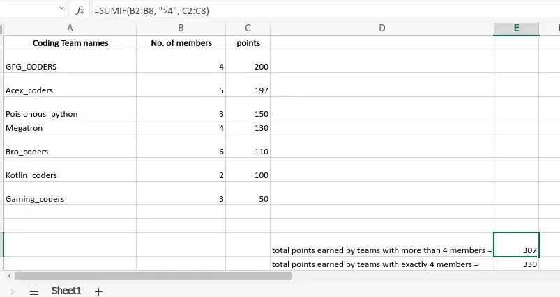
An Excel sheet has been taken as an example and the SUMIF function has been used in several formats.
Input:
| Coding Team names(Column A) | No. of members(Column B) | points(Column C) |
|---|
| GFG_CODERS | 4 | 200 |
|---|
| Acex_coders | 5 | 197 |
|---|
| Poisionous_python | 3 | 150 |
|---|
| Megatron | 4 | 130 |
|---|
| Bro_coders | 6 | 110 |
|---|
| Kotlin_coders | 2 | 100 |
|---|
| Gaming_coders | 3 | 50 |
|---|
Then we will apply the SUMIF() function to the above table:
| SUMIF() function | What the function does | Output result |
|---|
| =SUMIF(B2:B8, ">4", C2:C8) | If the no. of members in column B is greater than 4 then add the corresponding points of column C. | 307 |
|---|
| =SUMIF(B2:B8, 4, C2:C8) | If the no. of members in column B is equal to 4 then add the corresponding points of column C. | 330 |
|---|
| =SUMIF(A2:A8, "GFG_CODERS", C2:C8) | Search for "GFG_CODERS" in column A and add the corresponding points in column C. | 200 |
|---|
| =SUMIF(C2:C8, ">110") | Here the sum_range argument is not provided. So it will check the cells of C column and if the points are greater than 110 add it to the result. | 677 |
|---|
| =SUMIF(A2:A8, "*rs", C2:C8) | Here it will find the names of the teams ending with "rs" / "RS" in column A and add the corresponding points to the sum. | 657 |
|---|
Output:
 Output of Excel Sheet
- The Output after using the SUMIF Formula
 After Using the SUMIF Formula
How to Use SUMIFS with Multiple Criteria in Spreadsheet
Below are some examples of SUMIF Function in Excel:
Step 1: Enter the data Set
 Enter the Data Set
=SUMIFS(sum_range, criteria_range1, criteria1, [criteria_range2, criteria2], ...)
- sum_range: The range to add.
- criteria_range1, criteria1: The first range and condition pair.
- [criteria_range2, criteria2] (optional): Additional ranges and conditions.
Example : To sum the Sales where Product is "Product A" and Category is "Electronics":
=SUMIFS(C2:C10, A2:A10, "Product A", B2:B10, "Electronics")
 Enter the Formula
Conclusion
The SUMIF function is an essential tool for anyone working with data in Excel, allowing you to add up values based on specific criteria quickly. With a solid understanding of its syntax and practical applications, you’re now equipped to use SUMIF in various scenarios, from tracking budgets to analyzing sales. Start using SUMIF in your projects to save time and improve the accuracy of your data analysis!
Similar Reads
How to use IRR Function in Excel: Formula + Examples
How to Calculate Internal Rate of Return in Excel: Quick StepsEnter Your Cash FlowsEnter IRR Formula >> Press Enter Preview ResultsEver wondered how businesses decide which projects are worth investing in? The Internal Rate of Return (IRR) is a key financial metric that helps evaluate the prof
8 min read
Excel Date Functions with Formula Examples
There are many functions in Microsoft Excel that may be used to work with dates and timings in Excel. Each function completes a straightforward task, but by combining numerous functions into a single formula, you may handle trickier and more complicated problems. The purpose of discussing DATE funct
12 min read
How to Use HLOOKUP in Excel (Formula & Examples)
Excel HLOOKUP Function - Quick StepsSelect the cell Enter the HLOOKUP formulaInput arguments>>Press Enter Excel is packed with features that make handling and analyzing data easier. One of these handy tools is the HLOOKUP function, which is great for finding information in tables that are orga
9 min read
How to Combine Excel Functions in a Formula?
We all use Excel for some small computations in data but excel also provides the functionality to combine these small functions and make a formula for manipulating the data. For example, let's say that in school we need to increment the ID numbers of students by a number but the ID's have some text
2 min read
How To Use MATCH Function in Excel (With Examples)
Finding the right data in large spreadsheets can often feel like searching for a needle in a haystack. This is where the MATCH function in Excel proves invaluable. The MATCH function helps you locate the position of a specific value within a row or column, making it a cornerstone of efficient data m
6 min read
How to Create an Excel Step Chart Formula Using the Small Function?
A step Chart is a kind of line chart which uses horizontal and vertical lines to connect two different data points and forms a step-like structure. Unlike a line chart, it does not use the shortest distance to connect two different data points. A step chart is used to display data that varies uneven
3 min read
Top Excel Formulas and Functions You Should Know 2024
In the ever-evolving world of data analysis, mastering the top Excel formulas and functions is essential for maximizing productivity and efficiency. As we move into 2024, Excel remains a cornerstone tool for professionals across industries, from finance to marketing so for a better output you have t
15+ min read
How to use Conditional Formatting in Excel?
Microsoft Excel is a software that allows users to store or analyze the data in a proper systematic manner. It uses spreadsheets to organize numbers and data with formulas and functions. MS Excel has a collection of columns and rows that form a table. Generally, alphabetical letters are assigned to
4 min read
How to use CHOOSE Function in Excel
The CHOOSE function is technically part of Excel’s lookup function and can be incredibly useful. The CHOOSE function returns a value from a list using an index. One of those Excel features, CHOOSE, may not seem helpful alone, but when paired with other functions, it offers a ton of fantastic advanta
7 min read
Excel ROWS and COLUMNS Functions with Examples
In Microsoft Excel, where precision and efficiency reign supreme, mastering the art of maneuvering through cells and worksheets is indispensable. Two indispensable components in your Excel toolbox are the ROW and COLUMN functions, each meticulously crafted to execute discrete functions that can subs
7 min read