Single Layer Perceptron in TensorFlow
Last Updated :
11 Aug, 2025
Single Layer Perceptron is inspired by biological neurons and their ability to process information. To understand the SLP we first need to break down the workings of a single artificial neuron which is the fundamental building block of neural networks. An artificial neuron is a simplified computational model that mimics the behavior of a biological neuron. It takes inputs, processes them and produces an output. Here's how it works step by step:
- Receive signal from outside.
- Process the signal and decide whether we need to send information or not.
- Communicate the signal to the target cell, which can be another neuron or gland.
 Structure of a biological neuron
Similarly, neural networks also function in a similar manner.
 Neural Network in Machine Learning
Single Layer Perceptron
It is one of the oldest and first introduced neural networks. It was proposed by Frank Rosenblatt in 1958. Perceptron is also known as an artificial neural network. Perceptron is mainly used to compute the logical gate like AND, OR and NOR which has binary input and binary output.
The main functionality of the perceptron is:-
- Takes input from the input layer
- Weight them up and sum it up.
- Pass the sum to the nonlinear function to produce the output.
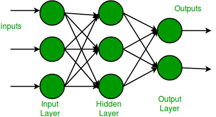
 Single-layer neural network
Here activation functions can be anything like sigmoid, tanh, relu based on the requirement we will be choosing the most appropriate nonlinear activation function to produce the better result. Now let us implement a single-layer perceptron.
Implementation of Single-layer Perceptron
Let’s build a simple single-layer perceptron using TensorFlow. This model will help you understand how neural networks work at the most basic level.
Step1: Import necessary libraries
- Scikit-learn – Scikit-learn provides easy-to-use and efficient tools for data mining and machine learning, enabling quick implementation of algorithms for classification, regression, clustering, and more.
- TensorFlow – This is an open-source library that is used for Machine Learning and Artificial intelligence and provides a range of functions to achieve complex functionalities with single lines of code.
Python
import tensorflow as tf
from sklearn.datasets import make_classification
from sklearn.model_selection import train_test_split
from sklearn.preprocessing import StandardScaler
Step 2: Create and split synthetic dataset
We will create a simple 2-feature synthetic binary-classification dataset for our demonstration and then split it into training and testing.
Python
X, y = make_classification(
    n_samples=1000,
    n_features=2,
    n_informative=2,
    n_redundant=0,
    n_repeated=0,
    n_classes=2,
    random_state=42
)

X_train, X_test, y_train, y_test = train_test_split(X, y, test_size=0.2, random_state=42)
Step 3: Standardize the Dataset
Now standardize the dataset to enable faster and more precise computations. Standardization helps the model converge more quickly and often enhances accuracy.
Python
scaler = StandardScaler()
X_train = scaler.fit_transform(X_train)
X_test = scaler.transform(X_test)
Step 4: Building a neural network
Next, we build the single-layer model using a Sequential architecture with one Dense layer. The Dense(1) indicates that this layer contains a single neuron. We apply the sigmoid activation function, which maps the output to a value between 0 and 1, suitable for binary classification. The original perceptron used a step function that only gave 0 or 1 as output and trained differently. But modern models use sigmoid because it’s smooth and helps the model learn better with gradient-based methods. The input_shape=(2,) specifies that each input sample consists of two features.
Python
model = tf.keras.Sequential([
    tf.keras.layers.Dense(1, activation='sigmoid', input_shape=(2,))
])
Step 5: Compile the Model
Next, we compile the model using the Adam optimizer, which is a popular and efficient algorithm for optimizing neural networks. We use binary cross-entropy as the loss function, which is well-suited for binary classification tasks with sigmoid activation. Additionally, we track the model’s performance using accuracy as the evaluation metric during training and testing.
Python
model.compile(optimizer='adam',
              loss='binary_crossentropy',
              metrics=['accuracy'])
Step 6: Train the Model
Now, we train the model by iterating over the entire training dataset a specified number of times, called epochs. During training, the data is divided into smaller batches of samples, known as the batch size, which determines how many samples are processed before updating the model’s weights. We also set aside a fraction of the training data as validation data to monitor the model’s performance on unseen data during training.
Python
history = model.fit(X_train, y_train,
                    epochs=50,
                    batch_size=16,
                    validation_split=0.1,
                    verbose=0)
Step 7: Model Evaluation
After training we test the model's performance on unseen data.
Python
loss, accuracy = model.evaluate(X_test, y_test, verbose=0)
print(f"Test Accuracy: {accuracy:.2f}")
Output:
Test Accuracy: 0.88
Even with such a simple model we achieved close to 88% accuracy. That’s quite impressive for a neural network with just one layer. However for even better results we could add hidden layers or use more complex architectures like CNNs (Convolutional Neural Networks).
Explore
Python Fundamentals
Python Data Structures
Advanced Python
Data Science with Python
Web Development with Python
Python Practice