Bayesian Statistics & Probability

Bayesian statistics sees unknown values as things that can change and updates what we believe about them whenever we get new information. It uses Bayes’ Theorem to combine what we already know with new data to get better estimates. In simple words, it means changing our initial guesses based on the evidence we find. This ongoing update helps us deal with uncertainty and make smarter decisions as more information comes in.

For example, when flipping a coin, usual statistics say there’s a 50% chance of heads. But if you already know the coin might be heavier on one side, Bayesian statistics lets you use that knowledge to adjust the chance of heads.

Before we dive into Bayes’ Theorem, let us first understand conditional probability.

Conditional Probability

Conditional probability is the probability of an event occurring given that another event has already occurred. It is denoted by P(A∣B) read as "the probability of event A given event B".

Bayes' Theorem

Bayes' Theorem is a mathematical formula that describes how to update the probability of a hypothesis based on new evidence. In simple terms it allow us to calculate the posterior probability (updated belief) by combining the prior probability (prior belief) and the likelihood of observing the evidence.

Mathematically Bayes’ Theorem is expressed as:

Where:

• P(\theta|X) is the posterior probability the updated belief after observing the data.
• P(X|\theta)is the likelihood the probability of observing the data given the hypothesis.
• P(\theta) is the prior probability, our initial belief about the hypothesis before observing the data.
• P(X)is the marginal likelihood a normalizing constant that ensures the posterior probability sums to 1.

Bayesian Statistics Components

Bayesian statistics uses three key parts: the likelihood function, prior belief, and posterior belief. These help handle yes/no outcomes and let us update our beliefs as we get new information. Let us understand them one by one:

1. Likelihood Function

The Bernoulli likelihood function is used for binary outcomes like success or failure. Like if we are studying the probability of a customer clicking on an ad (success) or not clicking (failure) this function helps us identify how likely it is to observe specific data given the probability of success.

Mathematically the Bernoulli likelihood function is represented as:

P(X|\theta) = \theta^x \cdot (1 - \theta)^{1 - x}

Where:

• X represents the observed data (0 for failure and 1 for success).
• \theta is the probability of success (e.g., click rate).
• x is the observed outcome (0 for failure, 1 for success).

2. Prior Distribution

Before we observe any data we have some prior beliefs about the parameters that we are estimating. For example we might have an initial belief that the probability of a customer clicking on an ad is around 0.3. The prior belief distribution reflects this knowledge. A commonly used probability parameter is the Beta distribution which is used as the prior distribution for parameters like \theta.

The prior belief distribution is mathematically expressed as:

P(\theta) = \frac{\theta^{\alpha - 1} \cdot (1 - \theta)^{\beta - 1}}{B(\alpha, \beta)}

Where:

• \theta represents the probability of success.
• \alpha and \beta are parameters that control the shape of the Beta distribution.
• B(\alpha, \beta) is the Beta function which ensures the distribution integrates to 1.

3. Posterior Distribution

Once new data is available we use Bayes’ Theorem to update our beliefs. The updated belief is represented by the posterior belief distribution which combines the prior belief and the new evidence.

P(\theta|X) \propto P(X|\theta) \times P(\theta)

The posterior distribution shows the updated probability of success or failure after we observe the data. As we receive new data our beliefs about the parameter will change accordingly

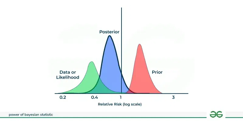
This graph explains how Bayesian statistics update our understanding of relative risk by combining prior beliefs with new data.

• The green curve represents the data which suggests the possible values for the risk based on observations.
• The red curve is the prior which show our belief about the risk before seeing the data.
• The blue curve is the posterior which is the updated belief after combining both.
• A steeper posterior means the data has a stronger influence while a flatter posterior means the prior has more more effect.

Example of Bayesian Statistics and Probability

Suppose a patient takes a test for a disease that affects 5% of the population (prior probability = 0.05).

The test results depend on:

• Sensitivity: 95% chance of a positive result if the patient has the disease.
• False Negative Rate: 5% chance of a negative result despite having the disease.
• False Positive Rate: 10% chance of a positive result without the disease.
• Specificity: 90% chance of a negative result if the patient is healthy.

The patient tests positive. Using Bayes’ Theorem, we update our belief about the patient having the disease:

P(\text{Disease}|\text{Positive}) = \frac{P(\text{Positive}|\text{Disease}) \times P(\text{Disease})}{P(\text{Positive})}

Where:

P(\text{Positive}) = P(\text{Positive}|\text{Disease}) \times P(\text{Disease}) + P(\text{Positive}|\text{No Disease}) \times P(\text{No Disease})

This calculation helps estimate the true chance the patient has the disease after the positive test.

Why Not Frequentist Approach?

The confusion between frequentist and Bayesian approaches has been constant for beginners. It's important to find the difference between these methods:

• Frequentist statistics relies solely on observed data and long-term frequencies, often ignoring prior knowledge. It uses point estimates and hypothesis testing with p-values, which can lead to rigid decisions.
• Bayesian statistics incorporates prior beliefs and updates them as data accumulates, offering more nuanced probability statements. This is especially useful for unique events or when data is limited.

Practical Use-Cases of Bayesian Statistics and Probability

• Spam Filtering: Bayesian filters learn from email characteristics to classify messages as spam or not.
• Marketing & Recommendations: Personalized suggestions are made by continuously updating user preference models.
• Probabilistic Modeling: Bayesian methods capture uncertainty in data and model parameters, useful in finance and customer behavior analysis.
• Bayesian Linear Regression: Unlike classical regression, it estimates distributions over coefficients, helpful with small or noisy datasets.
• A/B Testing: Provides full probability distributions over outcomes, offering richer insights than simple p-values.