Autoencoders in Machine Learning
Last Updated :
12 Jul, 2025
Autoencoders are a special type of neural networks that learn to compress data into a compact form and then reconstruct it to closely match the original input. They consist of an:
- Encoder that captures important features by reducing dimensionality.
- Decoder that rebuilds the data from this compressed representation.
The model trains by minimizing reconstruction error using loss functions like Mean Squared Error or Binary Cross-Entropy. These are applied in tasks such as noise removal, error detection and feature extraction where capturing efficient data representations is important.
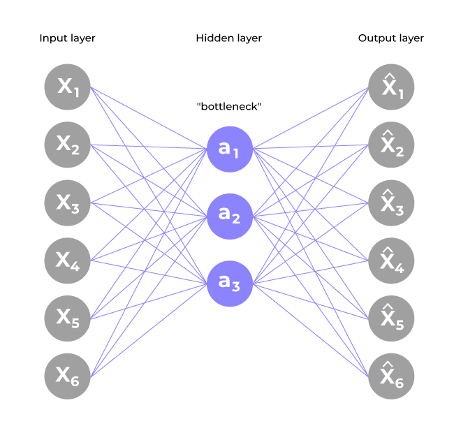
Architecture of Autoencoder
An autoencoder’s architecture consists of three main components that work together to compress and then reconstruct data which are as follows:
1. Encoder
It compress the input data into a smaller, more manageable form by reducing its dimensionality while preserving important information. It has three layers which are:
- Input Layer: This is where the original data enters the network. It can be images, text features or any other structured data.
- Hidden Layers: These layers perform a series of transformations on the input data. Each hidden layer applies weights and activation functions to capture important patterns, progressively reducing the data's size and complexity.
- Output(Latent Space): The encoder outputs a compressed vector known as the latent representation or encoding. This vector captures the important features of the input data in a condensed form helps in filtering out noise and redundancies.
2. Bottleneck (Latent Space)
It is the smallest layer of the network which represents the most compressed version of the input data. It serves as the information bottleneck which force the network to prioritize the most significant features. This compact representation helps the model learn the underlying structure and key patterns of the input helps in enabling better generalization and efficient data encoding.
3. Decoder
It is responsible for taking the compressed representation from the latent space and reconstructing it back into the original data form.
- Hidden Layers: These layers progressively expand the latent vector back into a higher-dimensional space. Through successive transformations decoder attempts to restore the original data shape and details
- Output Layer: The final layer produces the reconstructed output which aims to closely resemble the original input. The quality of reconstruction depends on how well the encoder-decoder pair can minimize the difference between the input and output during training.
Loss Function in Autoencoder Training
During training an autoencoder’s goal is to minimize the reconstruction loss which measures how different the reconstructed output is from the original input. The choice of loss function depends on the type of data being processed:
- Mean Squared Error (MSE): This is commonly used for continuous data. It measures the average squared differences between the input and the reconstructed data.
- Binary Cross-Entropy: Used for binary data (0 or 1 values). It calculates the difference in probability between the original and reconstructed output.
During training the network updates its weights using backpropagation to minimize this reconstruction loss. By doing this it learns to extract and retain the most important features of the input data which are encoded in the latent space.
Efficient Representations in Autoencoders
Constraining an autoencoder helps it learn meaningful and compact features from the input data which leads to more efficient representations. After training only the encoder part is used to encode similar data for future tasks. Various techniques are used to achieve this are as follows:
- Keep Small Hidden Layers: Limiting the size of each hidden layer forces the network to focus on the most important features. Smaller layers reduce redundancy and allows efficient encoding.
- Regularization: Techniques like L1 or L2 regularization add penalty terms to the loss function. This prevents overfitting by removing excessively large weights which helps in ensuring the model to learns general and useful representations.
- Denoising: In denoising autoencoders random noise is added to the input during training. It learns to remove this noise during reconstruction which helps it focus on core, noise-free features and helps in improving robustness.
- Tuning the Activation Functions: Adjusting activation functions can promote sparsity by activating only a few neurons at a time. This sparsity reduces model complexity and forces the network to capture only the most relevant features.
Types of Autoencoders
Lets see different types of Autoencoders which are designed for specific tasks with unique features:
1. Denoising Autoencoder
Denoising Autoencoder is trained to handle corrupted or noisy inputs, it learns to remove noise and helps in reconstructing clean data. It prevent the network from simply memorizing the input and encourages learning the core features.
2. Sparse Autoencoder
Sparse Autoencoder contains more hidden units than input features but only allows a few neurons to be active simultaneously. This sparsity is controlled by zeroing some hidden units, adjusting activation functions or adding a sparsity penalty to the loss function.
3. Variational Autoencoder
Variational autoencoder (VAE) makes assumptions about the probability distribution of the data and tries to learn a better approximation of it. It uses stochastic gradient descent to optimize and learn the distribution of latent variables. They used for generating new data such as creating realistic images or text.
It assumes that the data is generated by a Directed Graphical Model and tries to learn an approximation to q_{\phi}(z|x) to the conditional property q_{\theta}(z|x) where \phi and \theta are the parameters of the encoder and the decoder respectively.
4. Convolutional Autoencoder
Convolutional autoencoder uses convolutional neural networks (CNNs) which are designed for processing images. The encoder extracts features using convolutional layers and the decoder reconstructs the image through deconvolution also called as upsampling.
Implementation of Autoencoders
We will create a simple autoencoder with two Dense layers: an encoder that compresses images into a 64-dimensional latent vector and a decoder that reconstructs the original image from this compressed form.
Step 1: Import necessary libraries
We will be using Matplotlib, NumPy, TensorFlow and the MNIST dataset loader for this.
Python
import numpy as np
import matplotlib.pyplot as plt
import tensorflow as tf
from tensorflow import keras
from tensorflow.keras import layers, losses
from tensorflow.keras.models import Model
from keras.datasets import mnist
Step 2: Load the MNIST dataset
We will be loading the MNIST dataset which is inbuilt dataset and normalize pixel values to [0,1] also reshape the data to fit the model.
Python
(x_train, _), (x_test, _) = mnist.load_data()

x_train = x_train.astype('float32') / 255.
x_test = x_test.astype('float32') / 255.

x_train = np.reshape(x_train, (len(x_train), 28, 28, 1))
x_test = np.reshape(x_test, (len(x_test), 28, 28, 1))
Output:
Shape of the training data: (60000, 28, 28)
Shape of the testing data: (10000, 28, 28)
Step 3: Define a basic Autoencoder
Creating a simple autoencoder class with an encoder and decoder using Keras Sequential model.
- layers.Input(shape=(28, 28, 1)): Input layer expecting grayscale images of size 28x28.
- layers.Dense(latent_dimensions, activation='relu'): Dense layer that compresses the input to the latent space using ReLU activation.
- layers.Dense(28 * 28, activation='sigmoid'): Dense layer that expands the latent vector back to the original image size with sigmoid activation.
Python
class SimpleAutoencoder(Model):
    def __init__(self, latent_dimensions):
        super(SimpleAutoencoder, self).__init__()
        self.encoder = tf.keras.Sequential([
            layers.Input(shape=(28, 28, 1)),
            layers.Flatten(),
            layers.Dense(latent_dimensions, activation='relu'),
        ])

        self.decoder = tf.keras.Sequential([
            layers.Dense(28 * 28, activation='sigmoid'),
            layers.Reshape((28, 28, 1))
        ])

    def call(self, input_data):
        encoded = self.encoder(input_data)
        decoded = self.decoder(encoded)
        return decoded
Step 4: Compiling and Fitting Autoencoder
Here we compile the model using Adam optimizer and Mean Squared Error loss also we train for 10 epochs with batch size 256.
- latent_dimensions = 64: Sets the size of the compressed latent space to 64.
Python
latent_dimensions = 64
autoencoder = SimpleAutoencoder(latent_dimensions)
autoencoder.compile(optimizer='adam', loss=losses.MeanSquaredError())

autoencoder.fit(x_train, x_train,
                epochs=10,
                batch_size=256,
                shuffle=True,
                validation_data=(x_test, x_test))
Output:
 Training
Step 5: Visualize original and reconstructed data
Now compare original images and their reconstructions from the autoencoder.
- encoded_imgs = autoencoder.encoder(x_test).numpy(): Passes test images through the encoder to get their compressed latent representations as NumPy arrays.
- decoded_imgs = autoencoder.decoder(encoded_imgs).numpy(): Reconstructs images by passing the latent representations through the decoder and converts them to NumPy arrays.
Python
encoded_imgs = autoencoder.encoder(x_test).numpy()
decoded_imgs = autoencoder.decoder(encoded_imgs).numpy()

n = 6
plt.figure(figsize=(12, 6))
for i in range(n):
    ax = plt.subplot(2, n, i + 1)
    plt.imshow(x_test[i].reshape(28, 28), cmap='gray')
    plt.title("Original")
    plt.axis('off')

    ax = plt.subplot(2, n, i + 1 + n)
    plt.imshow(decoded_imgs[i].reshape(28, 28), cmap='gray')
    plt.title("Reconstructed")
    plt.axis('off')

plt.show()
Output:

The visualization compares original MNIST images (top row) with their reconstructed versions (bottom row) showing that the autoencoder effectively captures key features despite some minor blurriness.
Limitations of Autoencoders
Autoencoders are useful but also have some limitations:
- Memorizing Instead of Learning Patterns: It can sometimes memorize the training data rather than learning meaningful patterns which reduces their ability to generalize to new data.
- Reconstructed Data Might Not Be Perfect: Output may be blurry or distorted with noisy inputs or if the model architecture lacks sufficient complexity to capture all details.
- Requires a Large Dataset and Good Parameter Tuning: It require large amounts of data and careful parameter tuning (latent dimension size, learning rate, etc) to perform well. Insufficient data or poor tuning can result in weak feature representations.
Mastering autoencoders is important for applications in image processing, anomaly detection and feature extraction where efficient data representation is important.
Similar Reads
Deep Learning Tutorial Deep Learning is a subset of Artificial Intelligence (AI) that helps machines to learn from large datasets using multi-layered neural networks. It automatically finds patterns and makes predictions and eliminates the need for manual feature extraction. Deep Learning tutorial covers the basics to adv
5 min read
Deep Learning Basics
Introduction to Deep LearningDeep Learning is transforming the way machines understand, learn and interact with complex data. Deep learning mimics neural networks of the human brain, it enables computers to autonomously uncover patterns and make informed decisions from vast amounts of unstructured data. How Deep Learning Works?
7 min read
Artificial intelligence vs Machine Learning vs Deep LearningNowadays many misconceptions are there related to the words machine learning, deep learning, and artificial intelligence (AI), most people think all these things are the same whenever they hear the word AI, they directly relate that word to machine learning or vice versa, well yes, these things are
4 min read
Deep Learning Examples: Practical Applications in Real LifeDeep learning is a branch of artificial intelligence (AI) that uses algorithms inspired by how the human brain works. It helps computers learn from large amounts of data and make smart decisions. Deep learning is behind many technologies we use every day like voice assistants and medical tools.This
3 min read
Challenges in Deep LearningDeep learning, a branch of artificial intelligence, uses neural networks to analyze and learn from large datasets. It powers advancements in image recognition, natural language processing, and autonomous systems. Despite its impressive capabilities, deep learning is not without its challenges. It in
7 min read
Why Deep Learning is ImportantDeep learning has emerged as one of the most transformative technologies of our time, revolutionizing numerous fields from computer vision to natural language processing. Its significance extends far beyond just improving predictive accuracy; it has reshaped entire industries and opened up new possi
5 min read
Neural Networks Basics
What is a Neural Network?Neural networks are machine learning models that mimic the complex functions of the human brain. These models consist of interconnected nodes or neurons that process data, learn patterns and enable tasks such as pattern recognition and decision-making.In this article, we will explore the fundamental
12 min read
Types of Neural NetworksNeural networks are computational models that mimic the way biological neural networks in the human brain process information. They consist of layers of neurons that transform the input data into meaningful outputs through a series of mathematical operations. In this article, we are going to explore
7 min read
Layers in Artificial Neural Networks (ANN)In Artificial Neural Networks (ANNs), data flows from the input layer to the output layer through one or more hidden layers. Each layer consists of neurons that receive input, process it, and pass the output to the next layer. The layers work together to extract features, transform data, and make pr
4 min read
Activation functions in Neural NetworksWhile building a neural network, one key decision is selecting the Activation Function for both the hidden layer and the output layer. It is a mathematical function applied to the output of a neuron. It introduces non-linearity into the model, allowing the network to learn and represent complex patt
8 min read
Feedforward Neural NetworkFeedforward Neural Network (FNN) is a type of artificial neural network in which information flows in a single direction—from the input layer through hidden layers to the output layer—without loops or feedback. It is mainly used for pattern recognition tasks like image and speech classification.For
6 min read
Backpropagation in Neural NetworkBack Propagation is also known as "Backward Propagation of Errors" is a method used to train neural network . Its goal is to reduce the difference between the model’s predicted output and the actual output by adjusting the weights and biases in the network.It works iteratively to adjust weights and
9 min read
Deep Learning Models
Deep Learning Frameworks
TensorFlow TutorialTensorFlow is an open-source machine-learning framework developed by Google. It is written in Python, making it accessible and easy to understand. It is designed to build and train machine learning (ML) and deep learning models. It is highly scalable for both research and production.It supports CPUs
2 min read
Keras TutorialKeras high-level neural networks APIs that provide easy and efficient design and training of deep learning models. It is built on top of powerful frameworks like TensorFlow, making it both highly flexible and accessible. Keras has a simple and user-friendly interface, making it ideal for both beginn
3 min read
PyTorch TutorialPyTorch is an open-source deep learning framework designed to simplify the process of building neural networks and machine learning models. With its dynamic computation graph, PyTorch allows developers to modify the network’s behavior in real-time, making it an excellent choice for both beginners an
7 min read
Caffe : Deep Learning FrameworkCaffe (Convolutional Architecture for Fast Feature Embedding) is an open-source deep learning framework developed by the Berkeley Vision and Learning Center (BVLC) to assist developers in creating, training, testing, and deploying deep neural networks. It provides a valuable medium for enhancing com
8 min read
Apache MXNet: The Scalable and Flexible Deep Learning FrameworkIn the ever-evolving landscape of artificial intelligence and deep learning, selecting the right framework for building and deploying models is crucial for performance, scalability, and ease of development. Apache MXNet, an open-source deep learning framework, stands out by offering flexibility, sca
6 min read
Theano in PythonTheano is a Python library that allows us to evaluate mathematical operations including multi-dimensional arrays efficiently. It is mostly used in building Deep Learning Projects. Theano works way faster on the Graphics Processing Unit (GPU) rather than on the CPU. This article will help you to unde
4 min read
Model Evaluation
Deep Learning Projects