Disease prediction using machine learning is used in healthcare to provide accurate and early diagnosis based on patient symptoms. We can build predictive models that identify diseases efficiently. In this article, we will explore the end-to-end implementation of such a system.
Step 1: Import Libraries
We will import all the necessary libraries like pandas, Numpy, scipy, matplotlib, seaborn and scikit learn.
import numpy as np
import pandas as pd
from scipy.stats import mode
import matplotlib.pyplot as plt
import seaborn as sns
from sklearn.preprocessing import LabelEncoder
from sklearn.model_selection import train_test_split, cross_val_score, StratifiedKFold
from sklearn.svm import SVC
from sklearn.naive_bayes import GaussianNB
from sklearn.tree import DecisionTreeClassifier
from sklearn.ensemble import RandomForestClassifier
from sklearn.metrics import accuracy_score, confusion_matrix
from imblearn.over_sampling import RandomOverSampler
%matplotlib inline
Step 2: Reading the dataset
In this step we load the dataset and encode disease labels into numbers and visualize class distribution to check for imbalance. We then use RandomOverSampler to balance the dataset by duplicating minority classes and ensuring all diseases have equal samples for fair and effective model training.
You can download dataset from here : Click here.
data = pd.read_csv('/content/improved_disease_dataset.csv')

encoder = LabelEncoder()
data["disease"] = encoder.fit_transform(data["disease"])

X = data.iloc[:, :-1]
y = data.iloc[:, -1]

plt.figure(figsize=(18, 8))
sns.countplot(x=y)
plt.title("Disease Class Distribution Before Resampling")
plt.xticks(rotation=90)
plt.show()

ros = RandomOverSampler(random_state=42)
X_resampled, y_resampled = ros.fit_resample(X, y)
Output:

Step 3: Cross-Validation with Stratified K-Fold
We use Stratified K-Fold Cross-Validation to evaluate three machine learning models. The number of splits is set to 2 to accommodate smaller class sizes
if 'gender' in X_resampled.columns:
    le = LabelEncoder()
    X_resampled['gender'] = le.fit_transform(X_resampled['gender'])

X_resampled = X_resampled.fillna(0)

if len(y_resampled.shape) > 1:
    y_resampled = y_resampled.values.ravel()

models = {
    "Decision Tree": DecisionTreeClassifier(),
    "Random Forest": RandomForestClassifier(),
    "SVM": SVC()
}

cv_scoring = 'accuracy'  # you can also use 'f1_weighted', 'roc_auc_ovr' for multi-class
stratified_kfold = StratifiedKFold(n_splits=5, shuffle=True, random_state=42)

for model_name, model in models.items():
    try:
        scores = cross_val_score(
            model,
            X_resampled,
            y_resampled,
            cv=stratified_kfold,
            scoring=cv_scoring,
            n_jobs=-1,
            error_score='raise'
        )
        print("=" * 50)
        print(f"Model: {model_name}")
        print(f"Scores: {scores}")
        print(f"Mean Accuracy: {scores.mean():.4f}")
    except Exception as e:
        print("=" * 50)
        print(f"Model: {model_name} failed with error:")
        print(e)
Output:

The output shows the evaluation results for three models SVC, Gaussian Naive Bayes and Random Forest using cross-validation. Each model has two accuracy scores: 1.0 and approximately 0.976 indicating consistently high performance across all folds.
Step 4: Training Individual Models and Generating Confusion Matrices
After evaluating the models using cross-validation we train them on the resampled dataset and generate confusion matrix to visualize their performance on the test set.
Support Vector Classifier (SVC)
svm_model = SVC()
svm_model.fit(X_resampled, y_resampled)
svm_preds = svm_model.predict(X_resampled)

cf_matrix_svm = confusion_matrix(y_resampled, svm_preds)
plt.figure(figsize=(12, 8))
sns.heatmap(cf_matrix_svm, annot=True, fmt="d")
plt.title("Confusion Matrix for SVM Classifier")
plt.show()

print(f"SVM Accuracy: {accuracy_score(y_resampled, svm_preds) * 100:.2f}%")
Output:
SVM Accuracy: 60.53%

The matrix shows good accuracy with most values along the diagonal meaning the SVM model predicted the correct class most of the time.
nb_model = GaussianNB()
nb_model.fit(X_resampled, y_resampled)
nb_preds = nb_model.predict(X_resampled)

cf_matrix_nb = confusion_matrix(y_resampled, nb_preds)
plt.figure(figsize=(12, 8))
sns.heatmap(cf_matrix_nb, annot=True, fmt="d")
plt.title("Confusion Matrix for Naive Bayes Classifier")
plt.show()

print(f"Naive Bayes Accuracy: {accuracy_score(y_resampled, nb_preds) * 100:.2f}%")
Output:
Naive Bayes Accuracy: 37.98%

This matrix shows many off-diagonal values meaning the Naive Bayes model made more errors compared to the SVM. The predictions are less accurate and more spread out across incorrect classes.
rf_model = RandomForestClassifier(random_state=42)
rf_model.fit(X_resampled, y_resampled)
rf_preds = rf_model.predict(X_resampled)

cf_matrix_rf = confusion_matrix(y_resampled, rf_preds)
plt.figure(figsize=(12, 8))
sns.heatmap(cf_matrix_rf, annot=True, fmt="d")
plt.title("Confusion Matrix for Random Forest Classifier")
plt.show()

print(f"Random Forest Accuracy: {accuracy_score(y_resampled, rf_preds) * 100:.2f}%")
Output:
Random Forest Accuracy: 68.98%
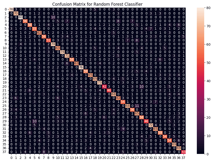
This confusion matrix shows strong performance with most predictions correctly placed along the diagonal. It has fewer misclassifications than Naive Bayes and is comparable or slightly better than SVM.
Step 5: Combining Predictions for Robustness
To build a robust model, we combine the predictions of all three models by taking the mode of their outputs. This ensures that even if one model makes an incorrect prediction the final output remains accurate.
from statistics import mode

final_preds = [mode([i, j, k]) for i, j, k in zip(svm_preds, nb_preds, rf_preds)]

cf_matrix_combined = confusion_matrix(y_resampled, final_preds)
plt.figure(figsize=(12, 8))
sns.heatmap(cf_matrix_combined, annot=True, fmt="d")
plt.title("Confusion Matrix for Combined Model")
plt.show()

print(f"Combined Model Accuracy: {accuracy_score(y_resampled, final_preds) * 100:.2f}%")
Output:
Combined Model Accuracy: 60.64%

Each cell shows how many times a true class (rows) was predicted as another class (columns) with high values on the diagonal indicating correct predictions.
Step 6: Creating Prediction Function
Finally, we create a function that takes symptoms as input and predicts the disease using the combined model. The input symptoms are encoded into numerical format and predictions are generated using the trained models.
symptoms = X.columns.values
symptom_index = {symptom: idx for idx, symptom in enumerate(symptoms)}

def predict_disease(input_symptoms):
    input_symptoms = input_symptoms.split(",")
    input_data = [0] * len(symptom_index)

    for symptom in input_symptoms:
        if symptom in symptom_index:
            input_data[symptom_index[symptom]] = 1

    input_df = pd.DataFrame([input_data], columns=symptoms)

    rf_pred = encoder.classes_[rf_model.predict(input_df)[0]]
    nb_pred = encoder.classes_[nb_model.predict(input_df)[0]]
    svm_pred = encoder.classes_[svm_model.predict(input_df)[0]]

    final_pred = mode([rf_pred, nb_pred, svm_pred])

    return {
        "Random Forest Prediction": rf_pred,
        "Naive Bayes Prediction": nb_pred,
        "SVM Prediction": svm_pred,
        "Final Prediction": final_pred
    }

print(predict_disease("skin_rash,fever,headache"))
Output:
{'Random Forest Prediction': 'Peptic ulcer disease', 'Naive Bayes Prediction': 'Impetigo', 'SVM Prediction': 'Peptic ulcer disease', 'Final Prediction': 'Peptic ulcer disease'}
This output shows that the Random Forest and SVM models both predict "Peptic ulcer disease", while the Naive Bayes model predicts "Impetigo" for the given symptoms. Since the majority of models agree on "Peptic ulcer disease," it is chosen as the final prediction. This suggests that "Peptic ulcer disease" is the most likely diagnosis based on the input symptoms according to the ensemble of models.
You can download source code from here.