Logistic Regression, as the name suggests is completely opposite in functionality. Logistic Regression is basically a predictive algorithm in Machine Learning used for binary classification. It predicts the probability of a class and then classifies it based on the predictor variables' values.
The dependent variable(y) in logistic regression, is binary and takes 2 possible values 0 or 1. For example: If we want to check if the mail is spam or not. Then y will have values - 1 for spam and 0 for not spam.
Logistic regression is analogous to linear regression in some aspects, just that in linear regression y is a continuous variable, whereas in logistic regression y needs to lie between 0 and 1. As, y is nothing but the predicted value and predicted value is nothing but the probability of y equals to 1, P(y = 1).
We know, the equation for linear regression:
Now, we know that this equation yields a continuous value of y. So as to restrict the predicted value of y in the 0 - 1 range, we apply the sigmoid function. The sigmoid function is,
Computing the value of y from the above equation and then putting in the linear regression equation, we get:
Hence, we finally get the equation for Logistic Regression. Using this equation, we can find the value of the probability of y when the value of x is known. In the above equation, b0 is the intercept and b1 is the slope matrix for all values of x. Collectively, we can refer to all as regression coefficients.
To learn more I will take the example of the Churn Modelling Data, a well-known dataset to predict a customer has churned out or not based on a number of features. Let's start with it in Julia.
Step 1: Import Packages
In this step, we will import all the required packages we will be using. Don't be afraid if you miss any package, you can definitely add it simultaneously.
# Import the packages
import Pkg;
Pkg.add("Lathe")
using Lathe

import Pkg;
Pkg.add("DataFrames")
using DataFrames

import Pkg;
Pkg.add("Plots")
using Plots;

import Pkg;
Pkg.add("GLM")
using GLM

import Pkg;
Pkg.add("StatsBase")
using StatsBase

import Pkg;
Pkg.add("MLBase")
using MLBase

import Pkg;
Pkg.add("ROCAnalysis")
using ROCAnalysis

import Pkg;
Pkg.add("CSV")
using CSV

println("Successfully imported the packages!!")
Output:
Successfully imported the packages!!
Step 2: Load the dataset
To read the data we use the CSV.file function and then convert it into data frame using DataFrame function.
# Load the data
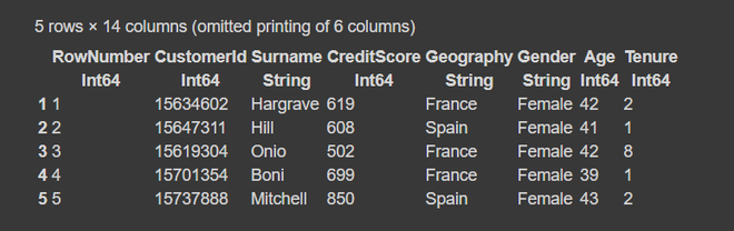
df = DataFrame(CSV.File("churn modelling.csv"))
first(df, 5)
Output:
Step 3: Summary of the dataframe
# Summary of dataframe
println(size(df))
describe(df)
Output:

The dependent variable, y in this case is the last column ('Exited'). The first column is just the row numbers and the variable from the second column are predictors or independent variables. Also, the size of our dataset is 10,000 rows and 14 columns. From the summary, we find that the dataset has no missing or null values. The column names don't have any spaces or special characters in them, hence we can go further without any problem.
select!(df, Not([:RowNumber, :CustomerId, :Surname, :Geography, :Gender]))
first(df, 5)
Output:

Step 4: Splitting the data into train and test set.
# Train test split
using Lathe.preprocess: TrainTestSplit
train, test = TrainTestSplit(df, .75);
Step 5: Building our Logistic Regression model.
We use the glm function for logistic regression.
# Train logistic regression model
fm = @formula(Exited ~ CreditScore + Age + Tenure +
              Balance + NumOfProducts + HasCrCard +
              IsActiveMember + EstimatedSalary)
logit = glm(fm, train, Binomial(), ProbitLink())
Output:

Once, we have built our model and trained it, we would evaluate the model on test data to see how accurately it works.
Step 6: Model prediction and evaluation
# Predict the target variable on test data
prediction = predict(logit, test)
Output:

The glm model gives us the probability score of class 1. After getting the probability score we need to classify it as 0 or 1 based n the threshold score. Usually, the threshold is considered 0.5.
With the help of the above code, we got the probability scores. Now, let's convert these into classes 0 or 1. For probability > 0.5 will be given class 1, otherwise 0.
# Converting probability score to classes
prediction_class = [if x < 0.5 0 else 1 end for x in prediction];

prediction_df = DataFrame(y_actual = test.Exited,
                          y_predicted = prediction_class,
                          prob_predicted = prediction);
prediction_df.correctly_classified = prediction_df.y_actual .== prediction_df.y_predicted
Output:

After, predicting the classes of our test data, the next step is to evaluate the model by analyzing the accuracy.
Step 7: Calculating the Accuracy of the model
By Accuracy, we mean the total number of classes our model predicted correctly.
# Finding the Accuracy Score
accuracy = mean(prediction_df.correctly_classified)
Output:
0.7996820349761526
So, our model yields an accuracy of approximately 80% which is a good score. Now, to get better insights of accuracy we analyze the confusion matrix.
Step 8: Confusion Matrix
The confusion matrix is just another way to evaluate the performance of any classification model.
# confusion matrix
confusion_matrix = MLBase.roc(prediction_df.y_actual,
                              prediction_df.y_predicted)
Output:
ROCNums{Int64}
  p = 523
  n = 1993
  tp = 69
  tn = 1943
  fp = 50
  fn = 454
The above output informs us that due to class imbalance our model classifies maximum observations as class 0. This is the reason for a moderate accuracy of 80%.