How to Calculate Internal Rate of Return in Excel: Quick Steps
- Enter Your Cash Flows
- Enter IRR Formula >> Press Enter
- Preview Results
Ever wondered how businesses decide which projects are worth investing in? The Internal Rate of Return (IRR) is a key financial metric that helps evaluate the profitability of investments. But calculating it manually can be tricky—thankfully, Excel’s IRR function makes it easy. Whether you’re analyzing uneven cash flows, comparing multiple projects, or just learning about financial metrics, this guide will show you how to calculate IRR in Excel step by step.
In this article, we’ll break down the Excel IRR formula with examples, explain the difference between IRR vs. NPV, and even cover advanced calculations like XIRR and MIRR. By the end, you’ll know how to use the IRR function like a pro and make smarter investment decisions.

Table of Content
- What Is Internal Rate of Return (IRR)
- Formula for Calculating Internal Rate of Return (IRR) in Excel
- How to Calculate IRR in Microsoft Excel: Step by Step Guide
- How to use XIRR Function in Excel (IRR for Irregular Cash Flows)
- How to use MIRR Function in Excel (Modified Internal Rate of Return)
- Example 1: Calculate IRR with Uneven Cash Flows
- Example 2: IRR for Multiple Projects
- Shortcut Keys for IRR, XIRR, and MIRR in Excel
- How to Fix if XIRR, IRR, and MIRR Errors in Excel
- Limitations of the IRR Function
- Tips for Using the IRR Function
What Is Internal Rate of Return (IRR)
The Internal Rate of Return (IRR) is the annualized rate of return at which the Net Present Value (NPV) of all cash flows (both positive and negative) from an investment equals zero. It’s commonly used to compare the profitability of different investments or projects.
- IRR > Required Rate of Return: The investment is profitable.
- IRR < Required Rate of Return: The investment is not profitable.
Why Use the IRR Function in Excel
- Easy Calculation: Automates complex IRR calculations.
- Compare Investments: Evaluate multiple projects or investments side by side.
- Decision-Making: Helps determine whether to proceed with a project or investment.
Net Present Value vs Internal Rate of Return
Net Present Value (NPV) and Internal Rate of Return (IRR) are both used to evaluate investment profitability, but they serve different purposes:
- NPV calculates the net value of future cash flows in today's terms using a discount rate. It helps determine if an investment will increase value.
- IRR finds the discount rate where NPV = 0, showing the expected annual return on an investment. It is useful for comparing project profitability.
For a detailed comparison, check out Difference between NPV and IRR.
Formula for Calculating Internal Rate of Return (IRR) in Excel
The syntax for the IRR function in Excel is:
=IRR(values, [guess])- values: A range of cash flows (must include at least one negative and one positive value).
- guess (optional): An estimated guess for the IRR (default is 10%).
How to Calculate IRR in Microsoft Excel: Step by Step Guide
The Internal Rate of Return (IRR) is a financial metric used to evaluate the profitability of investments. Excel’s IRR function makes it easy to calculate IRR. Here’s a quick step-by-step guide to calculate basic IRR Calculation.
Step 1: Enter Cash Flow Data in Excel
- List all cash flows in a column, including the initial investment (as a negative value).
Example:

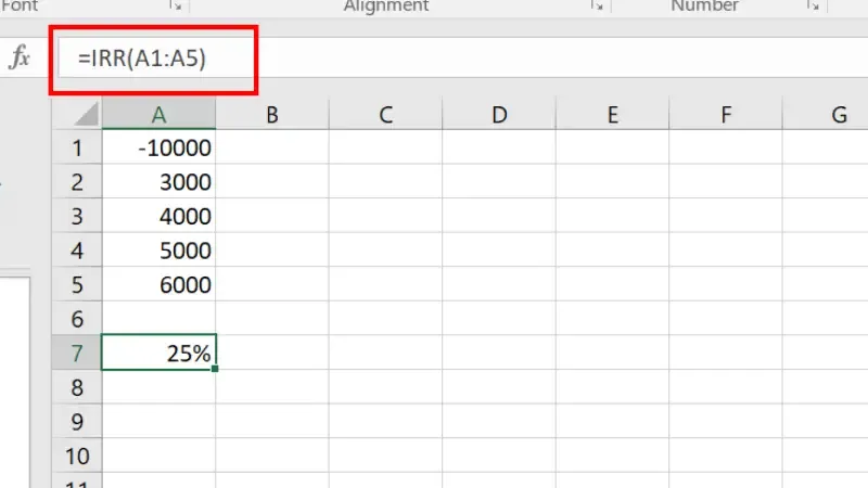
Step 2: Use the IRR Formula
- In a blank cell, enter the formula:
=IRR(A1:A5)A1:A5: The range of cash flows.
Step 3: Press Enter & Preview Results
- Excel will calculate and display the IRR as a percentage.
- Result: 25%
How to use XIRR Function in Excel (IRR for Irregular Cash Flows)
XIRR (Extended Internal Rate of Return) is a financial function used to calculate the annualized return of irregular cash flows over time. Unlike IRR, which assumes equal time gaps between cash flows, XIRR accounts for actual dates, making it more accurate for real-world investments.
When to Use XIRR
- When cash flows occur on different dates (e.g., investments, SIPs, loan repayments).
To measure the true return on investments in stocks, mutual funds, or private equity.
For personal finance planning when tracking irregular deposits and withdrawals.
Follow the below steps to calculate IRR Function in Excel:
For Example: A venture capitalist invests $50,000 in a startup and receives cash returns at different times:
Step 1: Enter the Data into the Sheet
Enter the Data into the Sheet. Date in Column A and cash flows in Column B.

Step 2: Enter the Formula
In an empty cell, write the formula.
=XIRR(B2:B5, A2:A5)
Step 3: Press Enter and Preview Results
Excel returns 18.9%, meaning the investment has an annualized return of 18.9%.

How to use MIRR Function in Excel (Modified Internal Rate of Return)
MIRR (Modified Internal Rate of Return) is an improved version of IRR (Internal Rate of Return) that considers both the cost of investment and the reinvestment rate of cash flows. This makes MIRR more realistic for evaluating project profitability.
You can easily calculate MIRR in Excel using the built-in MIRR Function. Here are the following steps to calculate MIRR in Excel:
Example: A company invests $100,000 in expanding its operations with varying annual returns. The company borrows at 8% and reinvests at 10%.
Step 1: Enter the Data
Enter the year in Column A and cash flows in Column B.

Step 2: Assume
- Finance rate = 8%
- Reinvestment rate = 10%
Step 3: Use the Below Formula
In the blank cell, use the below formula:
=MIRR(B2:B6, D3, D4)Step 4: Preview Results
Press Enter and Preview Results. Excel returns 18%, showing a more realistic return than standard IRR

Example 1: Calculate IRR with Uneven Cash Flows
Scenario: You have irregular cash flows over five years.
Step 1: Enter the Data into the Sheet
Enter the cash flows in a column

Step 2: Enter the Formula and Press Enter
In a blank cell, enter the formula:
=IRR(A2:A6)
Step 3: Preview Result
Preview the Result that is 23%.

Example 2: IRR for Multiple Projects
Scenario: Compare two projects to determine which is more profitable.
Step 1: Enter Cash Flows
Enter cash flows for Project A and Project B

Step 2: Enter the Formula
Select a Blank Cell and Enter the Formula
=IRR(A2:A6)=IRR(B2:B6)Step 3: Preview Results
Preview the Results that is:
- For Project A: 22%
- For Project B: 24%
Conclusion: Project B has a higher IRR and is more profitable.

Shortcut Keys for IRR, XIRR, and MIRR in Excel
| Action | Shortcut Key |
|---|---|
| Open Formula Bar | F2 |
| Apply Formula | Enter |
| Open Function Wizard | Shift + F3 |
| Recalculate Formulas | F9 |
How to Fix if XIRR, IRR, and MIRR Errors in Excel
When working with XIRR, IRR, and MIRR functions in Excel, you may encounter various errors due to incorrect data formatting, missing values, or calculation issues. Below are some of the most common errors and their solutions to help you resolve them quickly..
1. Getting #NUM! Error
Reason: Incorrect cash flow order or missing dates.
Fix: Ensure dates are in chronological order.
2. XIRR Returns a Negative Value
Reason: Net cash inflows are less than the initial investment.
Fix: Verify that future cash flows are positive.
3. IRR Calculation Doesn't Converge
Reason: Multiple IRRs exist due to fluctuating cash flows.
Fix: Use MIRR, which provides a more stable return estimate.
Limitations of the IRR Function
- Multiple IRRs: Projects with alternating cash flows may have multiple IRRs.
- Reinvestment Assumption: IRR assumes reinvestment at the same rate, which may not be realistic.
- No Scale Consideration: IRR does not account for the size of the investment.
Tips for Using the IRR Function
- Use Consistent Cash Flows: Ensure cash flows are entered in chronological order.
- Include Initial Investment: Always include the initial investment as a negative value.
- Compare with NPV: Use IRR alongside NPV for better decision-making.
- Adjust Guess for Accuracy: If Excel returns an error, adjust the
guessvalue.
Conclusion
Mastering the IRR function in Excel is a game-changer for anyone involved in financial analysis or investment planning. With this step-by-step guide for the IRR function, you’ve learned how to calculate IRR in Excel, handle uneven cash flows with XIRR, and adjust for reinvestment rates using MIRR. You’ve also explored the differences between IRR vs. NPV and tackled common errors and limitations.
Whether you’re evaluating a single project or comparing multiple investments, the IRR formula is a powerful tool to measure profitability. Ready to put your new skills to work? Open Excel, follow the examples, and start making data-driven decisions today.