INDEX and MATCH With Multiple Criteria In Excel

Excel is a wonderful tool and helps you to perform difficult tasks easily by using the defined functions. One such function in MS Excel is INDEX and MATCH. INDEX and MATCH are two functions, but they are used combinedly to find a value using multiple criteria. In other words, you can look up and return values even if there are no unique values to look for.  The INDEX/MATCH formula can help you find data points quickly without involving any manual search for them and risk making mistakes. Here, we will understand the syntax and formula in full detail so that you can easily adjust the formula for your particular needs and find values using multiple criteria. There are two ways to use INDEX and MATCH with multiple criteria to find results.

INDEX and MATCH with Multiple Criteria using an Array

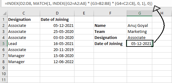
Consider the example (as shown below). Which contains information about the Employee's Name, Designation, Team, and Date of Joining.

And we need to find the Date of the Joining of Anuj Goyal who is a Marketing Associate in the company. Collect the prerequisites in the different cells (As shown below).

To find a value with multiple criteria in separate columns, use the generic formula below:

{=INDEX(return_range, MATCH(1, (criteria1=range1) * (criteria2=range2) * (…), 0))}

Where:

• Return_range is the range from which to return a value.
• Criteria1, criteria2, … are the conditions to be met.
• Range1, range2, … are the ranges on which the corresponding criteria should be tested.
   

Note: The above formula is an array formula and must be completed by pressing Ctrl + Shift + Enter together. This will enclose your formula in {curly brackets}, as shown, which is a visual sign of an array formula in Excel. If you try typing braces manually, that won't work! In our case the values are:

Return_range (Date of Joining) - D2:D8, Criteria1 (Name) - G2, Criteria2 (Team) - G3, Criteria3 (Designation) - G4, Range1 (Name) - A2:A8, Range2 (Team) - B2:B8, Range3 (Designation) - C2:C8
 

The complete formula is:

=INDEX(D2:D8, MATCH(1, (G2=A2:A8) * (G3=B2:B8) * (G4=C2:C8), 0))

Output:

After pressing Ctrl + Shift + Enter, you'll get the following output

INDEX and MATCH with Multiple Criteria Without using an Array

Considering the same example as used above. We need to find the Date of the Joining of Anuj Goyal who is a Marketing Associate in the company.

To find a value with multiple criteria without using arrays in separate columns, use the generic formula as below:

INDEX(return_range, MATCH(1, INDEX((criteria1=range1) * (criteria2=range2) * (..), 0, 1), 0))

According to our example the formula changes to:

=INDEX(D2:D8, MATCH(1, INDEX((G2=A2:A8) * (G3=B2:B8) * (G4=C2:C8), 0, 1), 0))

Explanation:  Return_range (Date of Joining) - D2:D8, Criteria1 (Name) - G2, Criteria2 (Team) - G3, Criteria3 (Designation) - G4, Range1 (Name) - A2:A8, Range2 (Team) - B2:B8, Range3 (Designation) - C2:C8. The INDEX function can handle arrays natively, the second INDEX is just used to "catch" the array formed by the boolean logic operation and return it to MATCH. INDEX is set up with zero rows and one column to do this. The zero-row technique causes INDEX to return column 1 from the array.

Output: After pressing Ctrl + Shift + Enter, you'll get the following output