The IF function in Google Sheets is one of the most versatile tools for logical testing and decision-making. Whether you’re working with numbers, text, or dates, this function allows you to evaluate conditions and define custom outputs based on whether those conditions are true or false. From simple comparisons to advanced nested formulas, mastering the IF function can significantly enhance your ability to automate tasks and analyze data.
This guide covers everything you need to know about using the IF function in Google Sheets, including practical examples, advanced use cases, and essential tips.
 Google Sheets IF Function
What is the IF Function in Google Sheets?
The IF function is a logical formula that evaluates a condition and returns a value if the condition is TRUE and another value if it’s FALSE.
IF Function Syntax
The IF function in Google Sheets follows a simple structure:
=IF(condition, value_if_true, value_if_false)
- condition: The logical test you want to evaluate (e.g., B2 > 50).
- value_if_true: The result to return if the condition is true.
- value_if_false: The result to return if the condition is false.
This syntax allows you to create flexible and dynamic formulas based on your data.
Example:
=IF(B2>50, "Pass", "Fail")
This formula checks if the value in B2 is greater than 50. If TRUE, it returns "Pass"; if FALSE, it returns "Fail."
Checking Equality with the IF Function
Use the IF function to determine if two values are equal. This is particularly useful for comparing targets, goals, or specific thresholds.
Example Scenario:
You have a spreadsheet where you're tracking sales commissions, and you want to check if a salesperson has met their target sales. If their sales are exactly $500, you want to display "Target Met"; otherwise, you'll show "Target Not Met".
Step 1: Set Up Your Data
- Input your data in Google Sheets.
- For example, enter sales figures in column B and add a column C for "Status."
 Set Up Your Data
- In C2 (under the "Status" column), type the following IF formula to check if the value in B2 (Sales Amount) is equal to 500:
=IF(B2=500, "Target Met", "Target Not Met")
 Write the Formula to Check for Equality
- After typing the formula, hit Enter.
- The formula will check if the value in B2 (Sales Amount) is exactly 500. If it is, it will return "Target Met". If not, it will return "Target Not Met".
Step 4: Apply to Other Rows
After pressing Enter, you will see "Target Met" for John (because his sales are 500) and "Target Not Met" for the other salespeople.
- To apply the formula to the other rows, drag the formula down:
- Click the small square handle at the bottom-right corner of C2.
- Drag the handle down to C5 (or however many rows you need).
Google Sheets will adjust the formula for each row (e.g., it will check B3, B4, and so on).
Example Output:
- For John: Since B2 = 500, the formula returns "Target Met".
- For Alice: Since B3 ≠ 500, the formula returns "Target Not Met".
- For Bob: Since B4 = 500, the formula returns "Target Met".
- For Sarah: Since B5 ≠ 500, the formula returns "Target Not Met".
 Apply to Other Rows
Using Greater Than or Less Than Conditions in IF
Check if a value is greater than or less than a specific number to automate grading, performance tracking, or data categorization.
Note: This is one of the best example of IF Function with Text
Step 1: Prepare Your Data
- Open Google Sheets.
- Select the cell where you want the result of the IF function to appear. This is the cell where Google Sheets will display "Pass" or "Fail" based on your condition (or any other custom output).
 Visit Google Sheets
- In the selected cell, start typing the formula with
=IF(. - The basic structure for the greater than condition is as follows:
=IF(condition, value_if_true, value_if_false)
For example, if you want to check if the value in cell B2 is greater than 50, you would write:
=IF(B2>50, "Pass", "Fail")
- Condition:
B2>50 (checks if the value in cell B2 is greater than 50). - Value if true: "Pass" (this value will be returned if the condition is true).
- Value if false: "Fail" (this value will be returned if the condition is false).
 Write the IF Formula
Step 3: Press Enter
- After typing the formula, press Enter to apply it.
- Google Sheets will evaluate the condition you set. If B2 is greater than 50, the formula will return "Pass". If B2 is 50 or less, it will return "Fail".
- You’ll see the result displayed in the selected cell based on the data in B2.
 Press Enter
To apply the formula to multiple rows or columns, you can drag and drop the formula to other cells.
- After entering the formula in one cell, place your cursor on the small square handle in the bottom-right corner of the cell.
- Click and drag the handle down or across to fill other cells with the same formula.
 Drag and Drop the Formula to Other Cells
The cell references will adjust automatically. For example, if you drag the formula down, it will apply the same greater than check to the next row (i.e., B3>50, B4>50, etc.).
Example Breakdown:
Here’s the full formula explained:
=IF(B1>50, "Pass", "Fail")
B1>50: This checks if the value in B1 is greater than 50."Pass": This is returned if the condition is true (i.e., B1 is greater than 50)."Fail": This is returned if the condition is false (i.e., B1 is less than or equal to 50).
Final Tips:
- You can replace "Pass" and "Fail" with other text or numerical values, depending on your needs. For example, you could return "Yes" or "No" instead.
- This method works well for conditions that compare numbers, like checking if sales, scores, or other numerical data meet certain thresholds.
- To make this even more dynamic, you can combine the IF function with other functions in Google Sheets, such as AND or OR, to evaluate more complex conditions.
- Using the drag and drop feature makes it easy to apply the formula to multiple rows or columns without having to re-enter it each time.
Nested IF Statements for Multiple Conditions
Use nested IF functions to evaluate multiple conditions, such as assigning grades or categorizing data into multiple tiers.
Step 1: Open Google Sheets and Choose the Cell
- First, launch Google Sheets and open the document where you want to use the multiple IF statements.
- Navigate to the cell where you want the result of your nested IF formula to appear. This is usually the cell where you want to display the final result after evaluating multiple conditions (e.g., "Grade" or "Category").
Choose a Cell In the selected cell, begin by typing the formula with =IF(. The IF function follows this syntax:
=IF(condition, value_if_true, value_if_false)
For example, if you're checking if a score (in cell B2) is greater than 90, you would write:
=IF(A1>90, "A",
 Start Writing the Formula
Step 3: Add Additional IF Statements
- To evaluate multiple conditions, you will nest another IF function inside the first one.
- After your first IF function, add a second IF function to check the next condition. For example, if you want to return "B" if the score is greater than 70 but less than or equal to 90, you would write:
=IF(B2>90, "A", IF(B2>70, "B", "C"))
In this case:
- If A1 is greater than 90, the formula returns "A".
- If A1 is not greater than 90 but is greater than 70, it returns "B".
- If neither condition is true, it returns "C".
 Add Additional IF Statements
Step 5: Apply the Formula
- Once you've written the entire formula with the conditions and the proper parentheses, press Enter.
- The formula will evaluate the data in cell A1, and based on the conditions you've set, it will return the appropriate result (either "A", "B", or "C").
- You can then drag the formula down to apply it to other cells in the column if necessary.
 Press Enter
Example Output:
Here’s the complete formula explained:
=IF(A1>90, "A", IF(A1>70, "B", "C")):
- If A1 > 90 → Returns "A".
- Else if A1 > 70 → Returns "B".
- Else → Returns "C".
This method of using nested IF functions allows you to evaluate multiple conditions and return different results based on those conditions. It’s particularly useful for situations where you need to categorize data or apply multiple thresholds, such as assigning grades or levels based on a numerical score.
Final Notes:
- Ensure Proper Syntax: Always double-check parentheses and commas to ensure there are no errors.
- Complex Conditions: For more complex formulas, consider using the
IFS function, which can handle multiple conditions without the need for nested IFs.
Combining IF with AND/OR for Multiple Criteria
Combine IF with AND/OR to evaluate multiple conditions simultaneously, such as checking for eligibility or qualifying conditions.
Step 1: Use AND for All Conditions
=IF(AND(B2>50, C2>75), "Pass", "Fail")
Checks if B2 > 50 and C2 > 75.
Step 2: Use OR for Any Condition
- Example Formula: =IF(OR(B2=0, C2="Discontinued"), "Unavailable", "Available")
- Checks if B2 is 0 or C2 is "Discontinued."
Step 3: Test the Results
Drag the formula down for all rows and verify the outcomes.
Using IF with Dates
Check if a date is overdue or falls within a specific range.
Enter due dates in column A.
To check if a task is overdue, enter: =IF(A2<TODAY(), "Overdue", "On Time")
Drag the formula to other rows to evaluate all dates.
Handling Empty Cells with IF
Use the IF function to check if a cell is empty or contains data. This is useful for tracking missing entries.
Step 1: Select a Cell
- Open Google Sheets and navigate to the spreadsheet where you want to use the IF function.
- Click on the cell where you want the result to appear. For example, if you are checking the status of email entries, select C2 (the first cell under the "Status" column).
 Open Google Sheets >> Select a Cell
In the selected cell (e.g., C2), type the IF formula to check if the "Email" cell (e.g., B2) is blank:
=IF(B2="", "Missing Email", "Email Provided")
- Condition:
B2="" checks if B2 is empty (i.e., contains no value). - Value if true:
"Missing Email" (this will be displayed if B2 is blank). - Value if false:
"Email Provided" (this will be displayed if B2 contains any value).
 Enter the Formula to Check Blanks
Step 3: Press Enter
- After typing the formula, press Enter to apply it.
- Google Sheets will evaluate the condition: if B2 is empty, the formula will return "Missing Email"; if B2 contains an email, it will return "Email Provided".
- You’ll see the result in C2.
 Press Enter
Step 4: Apply to Other Rows
To apply the formula to other rows in the "Status" column, drag the formula down from C2.
- Click the small square handle in the bottom-right corner of C2.
- Drag the handle down to fill the formula into the remaining cells in the "Status" column.
- The formula will adjust automatically for each row (e.g.,
B3="", B4="", etc.), so it checks the corresponding cell for each row.
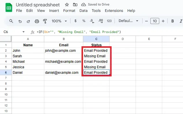 Apply to Others
 Example Breakdown:
Here’s the full formula explained:
=IF(B2="", "Missing Email", "Email Provided")
B2="": This checks if B2 is empty (blank)."Missing Email": This is returned if B2 is blank."Email Provided": This is returned if B2 is not blank.
Final Tips:
- You can customize the text in the formula. For example, instead of "Missing Email", you could display "No Email Found".
- The IF function is very flexible; you can combine it with other functions like AND or OR to check for multiple conditions (e.g., if both the email and name are missing).
- Drag and drop makes it easy to apply this formula to entire columns of data quickly without having to re-enter it.
By using the IF function to check for empty cells in Google Sheets, you can automatically flag missing information and keep your data clean and organized. This approach helps you ensure that you don’t overlook important details, such as missing email addresses, in your spreadsheet.
Preventing Errors with IFERROR
Combine IF with IFERROR to handle potential formula errors gracefully.
Use the formula:
=IFERROR(A2/B2, "Error: Division by Zero")
Enter zero in B2 to verify that the error is handled.
Tips for Using IF Function in Google Sheets
- Absolute References: Use
$ to lock cell references (e.g., $B$2) for consistent formulas. - Combine with Other Functions: Pair IF with SUM, COUNT, or AVERAGE for more dynamic calculations.
- Highlight Data: Use Conditional Formatting with IF to visually emphasize key results.
- Simplify Complex Conditions: Use IFS or combine IF with AND/OR for cleaner formulas.
Conclusion
The IF function in Google Sheets can simplify a wide range of tasks, from creating automated decision-making rules to calculating values based on specific conditions. Whether you're just getting started with basic formulas or exploring more complex nested functions, mastering the IF function will help you streamline your workflows and enhance your data analysis. By using the insights in this guide, you'll be able to create smarter, more efficient Google Sheets documents tailored to your unique needs.
Similar Reads
OR Logical Function in Google Sheets The OR function in Google Sheets is a versatile logical function that helps evaluate multiple conditions within your dataset. It is particularly useful in data analysis and decision-making, as it allows you to assess whether any given criteria are true. By combining it with other logical functions i
7 min read
Top Google Sheets Formulas Google Sheets is a versatile, cloud-based spreadsheet tool that allows users to create, edit, and share data online. Whether you're managing a business, organizing school work, or performing data analysis, learning Google Sheets formulas can significantly enhance your productivity. With the right fo
8 min read
Excel IF Function The IF function in Excel is one of the most powerful and commonly used formulas that allows you to perform logical tests and return different values based on whether the condition is true or false. If you’ve ever needed to check whether a value meets certain criteria, then the IF function is the too
12 min read
Google Sheets IF ELSE The IF ELSE function in Google Sheets is a powerful tool for making decisions based on specific conditions within your data. While the basic IF function allows you to specify one action for a "TRUE" condition and another for a "FALSE" condition, IF ELSE introduces more flexibility by enabling multip
10 min read