How to Freeze Top Row and First Column in Excel (2025 Updated)

When working with large datasets in Excel, it can be challenging to keep track of key headers and labels as you scroll through rows and columns. Fortunately, Excel provides a powerful feature called Freeze Panes, which allows you to lock specific rows, columns, or both in place, making it easier to analyze your data without losing context. In this article, we'll guide you through the process of freezing the Top Row and First Column in Excel, along with helpful tips and shortcuts.

Why Use Freeze Panes in Excel?

The Freeze Panes feature in Excel is useful for:

• Freezing the Top Row: Keeps the column headers visible while scrolling down through large datasets. This is especially helpful when you're working with tables where the headers identify each column's content, such as "Name," "Product ID," or "Sales Date."
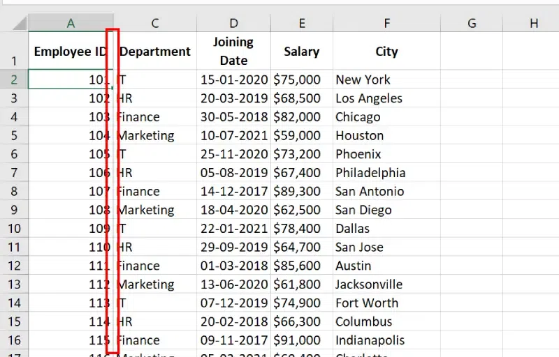
• Freezing the First Column: Ensures that important row labels or identifiers (such as "Employee ID," "Product Name," or "Category") stay visible as you scroll horizontally across the worksheet.

How to Freeze the Top Row in Excel

Freezing the top row ensures that the header row remains visible when scrolling down your worksheet. Follow these steps:

Step 1: Open Your Excel File

• Open the Excel workbook containing your data.
• Ensure that the first row contains the headers or labels you want to freeze, such as "Employee ID," "Name," "Department," etc.

Step 2: Go to the "View" Tab and Select "Freeze Panes"

• Click on the View tab in the Ribbon.
• In the Window group, click on the Freeze Panes dropdown.
• From the dropdown menu, select Freeze Top Row.

Alternatively, you can use the keyboard shortcut:

• Windows: Press Alt + W + F + R
• Mac: Press Command + Option + Shift + R

Step 3: Test by Scrolling Down

Scroll down your worksheet. You’ll notice that the top row remains visible while the rest of the data scrolls. This is especially useful when working with large datasets that have numerous rows.

How to Freeze the First Column in Excel

Freezing the first column ensures that key identifiers such as names, IDs, or product codes stay visible as you scroll horizontally across your worksheet.

Step 1: Open Your Excel File

• Open the Excel workbook with the data you want to work with.
• Ensure that the first column contains essential identifiers such as "Employee Name," "Product ID," or other key information.

Step 2: Go to the "View" Tab and Select "Freeze Panes"

• Click on the View tab in the Ribbon.
• In the Window group, click on the Freeze Panes dropdown.
• Select Freeze First Column.

Alternatively, use the keyboard shortcut:

• Windows: Press Alt + W + F + C
• Mac: Press Command + Option + Shift + C

Step 3: Test by Scrolling Horizontally

Scroll horizontally across your worksheet. You’ll notice that the first column stays visible while the rest of the data moves horizontally.

How to Freeze Both the Top Row and First Column in Excel

If you want to freeze both the Top Row and the First Column, follow these steps:

Step 1: Open Your Excel File

Open the Excel workbook where you want to freeze both the top row and first column.

Step 2: Select the Cell Below and to the Right of the Rows and Columns

Select the cell immediately below the top row and to the right of the first column. For example:

• For Example: If you want to freeze Row 1 and Column A, select cell B2.

Step 3: Go to the "View" Tab and Select "Freeze Panes"

• Click on the View tab in the Ribbon.
• In the Window group, click on the Freeze Panes dropdown.
• Select Freeze Panes (this option locks both the top row and the first column).

Alternatively, you can use the keyboard shortcut:

• Windows: Press Alt + W + F + F
• Mac: Press Command + Option + F

Step 4: Test by Scrolling

Scroll both vertically and horizontally. You’ll notice that the top row and first column remain visible while the rest of the worksheet scrolls.

Conclusion

Freezing the Top Row and First Column in Excel can significantly enhance your workflow, especially when working with large datasets. Whether you need to keep column headers in view while scrolling down or keep row labels visible as you scroll horizontally, the Freeze Panes feature is an invaluable tool for making your data easier to navigate and analyze. By following the steps outlined in this guide, you can quickly master freezing rows, columns, or both in Excel.