How to Create and Use Pivot Tables in Google Sheets
Last Updated :
30 Dec, 2024
Pivot tables in Google Sheets are indispensable for turning raw data into meaningful insights. Whether you’re tracking sales, analyzing marketing metrics, or managing financial data, pivot tables allow users to create dynamic data summaries with ease. This tutorial covers how to use pivot tables in Google Sheets, including creating them with multiple sheets and troubleshooting common issues. Professionals across industries like finance, marketing, and project management can significantly benefit from mastering this versatile tool.
What is a Pivot Table in Google Sheets
A Pivot Table in Google Sheets is a powerful tool for summarizing and analyzing large datasets. It dynamically reshapes data, allowing you to group, filter, and perform calculations like SUM, COUNT, or AVERAGE to extract meaningful insights. For Example, a sales team can use a Pivot Table to summarize monthly sales by product and region, filtering for specific timeframes to identify trends. Pivot Tables offer dynamic data summarization and efficient analysis, making them an essential tool for decision-making.
How to Create a Pivot Table in Google Sheets
Follow this Google Sheets pivot table tutorial to quickly make a Pivot Table:
Step 1: Select the Data Range
Highlight the data range you want to include in the pivot table. For example, select A2:D9.
 Open Google Sheets >> Select Data
Step 2: Open the Pivot Table Option
Go to the menu bar, click on Insert, and choose Pivot Table.
 Go to Insert Tab >> Select Pivot Table
 Step 3: Choose the Location for the Pivot Table
In the pop-up window, decide whether to place the pivot table in a new sheet or the existing one. Click Create.
 Choose Location >> Click on "Create" Button
Step 4: Add Rows to the Pivot Table
In the Pivot Table Editor, click Add under the Rows section. Select "Category" to group data by category (e.g., Electronics and Clothing).
 Add Rows to the Pivot Table
Step 5: Add Columns to the Pivot Table
Click Add under the Columns section and select "Region" to categorize data by region.
 Click on Add Button >> Add Columns
Step 6: Add Values to the Pivot Table
Click Add under the Values section and select "Sales." Ensure the summarization is set to "SUM" to display total sales.
 Add Values
 Step 7: Analyze the Pivot Table
Review the generated pivot table. It will summarize sales by category and region, helping you draw insights quickly.
 Analyze the Pivot Table
How to Create a Pivot Table from Multiple Sheets in Google Sheets
This Google Sheets pivot table tutorial will guide you on how to create a pivot table using data from multiple sheets. It allows you to combine and analyze data from different sources in one place. Ideal for scenarios like comparing sales data from different regions or departments stored in separate sheets.
Step 1: Organize Data in Separate Sheets
Ensure the data you want to include in the pivot table is spread across multiple sheets, like "Sales Data" in Sheet 1 and "Category Data" in Sheet 2.
To use data from multiple sheets in a pivot table, you must combine it into one sheet.
In a new sheet (e.g., Combined Data), use the QUERY function:
=QUERY({Sheet1!A2:C, Sheet2!B2:B}, "SELECT Col1, Col2, Col3, Col4") This combines the data into one table.
 Combine Data Using QUERY or ARRAYFORMULA
Step 3: Select the Data Range for the Pivot Table
Highlight the combined data in the new sheet, e.g., A1:D4.
 Select the Data Range
Step 4: Insert the Pivot Table
Go to the menu bar, click Insert, and select Pivot Table.
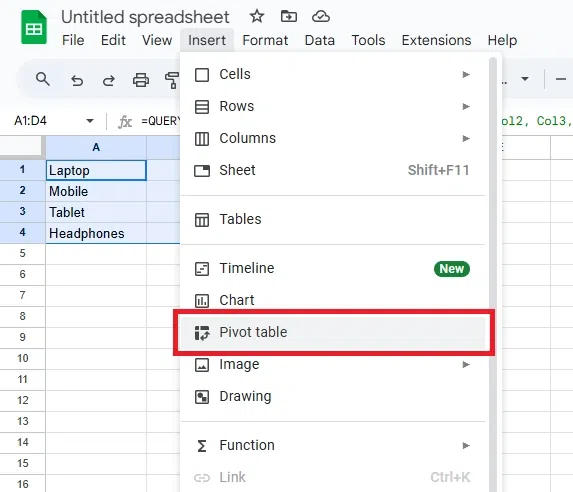 Go to Insert >> Select Pivot Table
Step 5: Choose the Location for the Pivot Table
In the pop-up window, choose whether to place the pivot table in a new sheet or the existing one, then click Create.
 Choose the Location >> Click "Create"
Step 6: Add Rows to the Pivot Table
In the Pivot Table Editor, click Add under the Rows section. Select "Category" to group data by product categories.
 Add Rows to the Pivot Table
Step 7: Add Columns to the Pivot Table
Click Add under the Columns section and select "Region" to categorize data by sales regions.
 Add Columns to the Pivot Table
Step 8: Add Values to the Pivot Table
Click Add under the Values section and select "Sales." Set the summarization to "SUM" to calculate total sales.
 Add Values to the Pivot Table
Troubleshooting Common Issues
Here are some common problems with Pivot Tables in Google Sheets and their solutions:
| Issue | Cause | Solution |
|---|
| Pivot Table Not Updating | Source data has changed but the pivot table hasn’t. | Click anywhere on the pivot table and press Refresh in the Pivot Table Editor. |
| Data Range Error | Incorrect or incomplete data range selected. | Check and update the data range by clicking Edit Data Range in the Pivot Table Editor. |
| Missing Data in Pivot Table | Blank cells or mismatched formatting in the source. | Ensure the source data is clean, with no blank rows or mismatched formats. |
| Duplicate Data Entries | Duplicate rows in the source dataset. | Remove duplicates using the Data > Remove Duplicates feature. |
| Cannot Group Data | Text data in a column intended for numerical grouping. | Convert text to numbers, or use a helper column with the correct format. |
| #REF! or #VALUE! Errors | Invalid formulas or references in the source data. | Fix errors in the source data before creating the pivot table. |
Tips for Preventing Issues
- Always keep your source data organized and properly formatted.
- Use filters to remove unnecessary data before creating the pivot table.
- Regularly refresh the pivot table to ensure it reflects the latest updates.
By addressing these issues, you can maintain smooth and accurate Pivot Table functionality in Google Sheets.
Also Read:
Conclusion
Mastering pivot tables in Google Sheets unlocks a powerful way to analyze and organize data. By using this guide, you can create pivot tables, summarize information across multiple sheets, and troubleshoot issues effectively. Take the time to explore these features further and discover how they can simplify complex data analysis in your daily work.
Similar Reads
How to Use Add-Ons in Google Sheets
Google Sheets add-ons offer an incredible way to expand the functionality of your spreadsheets, making them more efficient and versatile for various tasks. Whether you’re looking to automate repetitive workflows, perform advanced data analysis, or customize your sheets for specific needs, add-ons fr
3 min read
How to Use Data Bars in Google Sheets
Data bars in Google Sheets visually represent your data, making it easier to compare values within a range. By applying data bars through Conditional Formatting, you can instantly see trends, differences, and patterns in your dataset. This feature is especially useful for highlighting high or low va
5 min read
What Is Google Sheets and How to use it?
Google Sheets designed as part of Google Workspace (formerly G Suite), Google Sheets works seamlessly online, enabling users to manage data, perform calculations, and visualize information through charts and graphs. It is a popular alternative to Microsoft Excel, offering accessibility across device
5 min read
How to Create and Customize Pie Charts in Google Sheets
Pie charts are a powerful tool for visualizing data, offering a straightforward way to understand proportions and percentages at a glance. Perfect for breaking down categories in a dataset, they transform complex information into clear visuals. Google Sheets provides easy-to-use features to make a p
8 min read
How To Create A Timesheet In Google Docs
How To Create A Timesheet In Google Docs - Quick StepsOpen Google Docs > Go to InsertSelect Table > Specify Table SizeCustomize TableEnter Timesheet DataGet ready to take control of your time with Google Docs! Today, we're diving into the simple yet powerful world of creating a timesheet. Whet
6 min read
How To Split Table In Google Docs
Google Docs, a widely used word-processing software developed by Google, allows users to create, edit, and share documents online while collaborating with others in real-time. Splitting a table in Google Docs is a simple yet essential skill for anyone looking to organize and present information effe
3 min read
How to Prevent Grouped Dates In Excel Pivot Table?
We may group dates, numbers, and text fields in a pivot table. Organize dates, for instance, by year and month. In a pivot table field, text elements can be manually selected. The selected things can then be grouped. This enables you to rapidly view the subtotals in your pivot table for a certain gr
3 min read
How to Create a Power PivotTable in Excel?
When we have to compare the data (such as name/product/items, etc.) between any of the columns in excel then we can easily do with the help of Pivot table and pivot charts. But it fails when it comes to comparing those data which are in two different datasets, at that time Power Pivot comes into rol
4 min read
How to Sort a Pivot Table in Excel : A Complete Guide
Sorting a Pivot Table in Excel is a powerful way to organize and analyze data effectively. Whether you want to sort alphabetically, numerically, or apply a custom sort in Excel, mastering this feature allows you to extract meaningful insights quickly. This guide walks you through various Pivot Table
7 min read
How to Make Bar Charts in Google Sheets
Bar charts are an excellent way to visually represent data comparisons, and Google Sheets offers intuitive tools to create and customize them. Whether you're looking to create a bar graph in Google Sheets or explore options like grouped and stacked bar charts, this guide will walk you through the st
5 min read