How to Create a Waterfall Chart in Excel
Last Updated :
19 Dec, 2024
Waterfall charts are a powerful visualization tool used to illustrate the cumulative effect of sequential data points, such as profits, losses, or changes over time. Widely used in financial and performance analysis, these charts provide clear insights into the contributions of individual components to a total value. Whether you’re presenting a business report or analyzing operational results, a waterfall chart in Excel can make your data more comprehensible. This guide will cover how to create a waterfall chart in Excel, along with waterfall chart customization in Excel for tailoring visuals to your specific needs.
Disclaimer: Always ensure the accuracy of your data and double-check calculations to avoid misrepresentations in analysis.

Create a Waterfall Chart in Excel
How to Create a Waterfall Chart in Excel
Creating a Waterfall chart in Excel is simple and helps you visualize changes in values over time or categories. Follow these steps to create a waterfall diagram in Excel:
Note: Keep in mind that creating waterfall charts is easy in Excel 2016 and newer versions because they have a built-in option for it. In older versions, it’s more complicated and takes extra time since there isn’t a direct way to add a waterfall chart.
Step 1: Prepare Your Data
Organize your data in a table with categories and values. Include starting and ending totals, as well as gains and losses in between.
Ensure that positive values (e.g., sales) are entered as positive numbers and negative values (e.g., expenses) are entered with a minus sign.

Enter data into the sheet
Step 2: Insert the Waterfall Chart
Highlight the Data:
- Select the table, including both the Category and Values columns.
Insert Chart:
- Go to the Insert tab on the Excel ribbon.
- In the Charts group, click the Insert Waterfall or Stock Chart dropdown.
- Choose Waterfall from the options.

Insert>>Waterfall Chart
Step 3: Preview the Waterfall Diagram
Excel will automatically generate a basic Waterfall Chart based on your data.

Waterfall Chart Created
Customizing a Waterfall Chart in Excel
After learning how to create a waterfall chart in Excel, you can enhance its clarity and appeal with waterfall chart customization in Excel. Follow these steps:
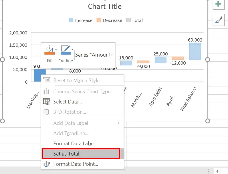
Step 1: Set the Starting and Final Balances as Totals
- Click on the Starting Balance bar in the chart.
- Right-click and select Set as Total. This will anchor the starting point of the chart to the baseline.
- Repeat the same steps for the Final Balance bar to mark it as the ending total.
Create a Waterfall Chart in Excel
Step 2: Adjust the Colors for Clarity
- Click on any bar representing a positive change (e.g., January Sales), then right-click and choose Format Data Series.
- Under the Fill & Line options, change the color to green (or another color representing a gain).
- For negative changes (e.g., January Expenses), change the color to red to indicate a loss.
- You can choose a different color for the Starting Balance and Final Balance bars to make them stand out (e.g., blue).

Change the color
Step 3: Add Data Labels
- Right-click on any bar in the chart.
- Select Add Data Labels to display the numerical values on the bars.
- Adjust the position of the labels (e.g., Above, Below) for better readability.
Step 4: Adjust the Gap Width (Optional)
- Click on any bar in the chart, right-click, and choose Format Data Series.
- Reduce the Gap Width to make the bars wider and improve the visual appearance.

Right-Click and Select Format Axis >> Adjust the Gap Width
Step 5: Add a Chart Title
Click on the chart title and change it to something descriptive, like “Company Profit Analysis – Waterfall Chart“.
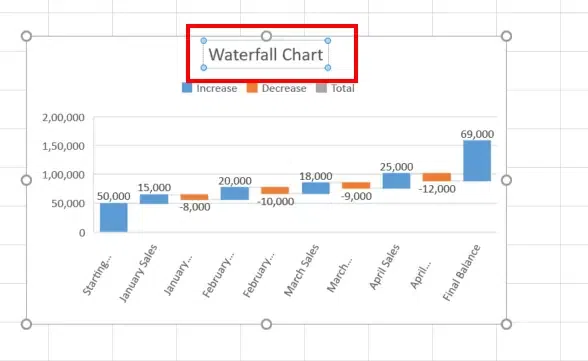
Add a Chart Tittle
Step 6: Modify the Y-Axis Scale if Needed
- Click on the Y-axis, right-click, and choose Format Axis.
- Adjust the minimum and maximum values for the Y-axis to better fit your data range.

Right – Click >> Modify the Y-Axis Scale
Step 7: Review and Save Your Work
- Review the final chart to ensure all details are correctly displayed.
- Save your Excel file to preserve the chart.

Review and Save your Work
The final waterfall chart will clearly show the financial journey from the starting balance to the final balance, with incremental gains and losses for each month displayed in between. This visualization helps you easily understand the impact of each financial event on the overall profit.
Also Read:
Conclusion
Creating a Waterfall chart in Excel is a straightforward way to analyze and visualize changes in values over time or across categories. This powerful tool helps you clearly identify contributions to totals, whether in financial data, performance metrics, or other key analyses. By knowing Excel’s built-in features, you can customize your chart to suit your needs and present data in an easy-to-understand format. Mastering the Waterfall chart will not only enhance your data analysis but also improve the clarity and impact of your presentations.
Similar Reads
How to Create a Waterfall Chart in Excel
Waterfall charts are a powerful visualization tool used to illustrate the cumulative effect of sequential data points, such as profits, losses, or changes over time. Widely used in financial and performance analysis, these charts provide clear insights into the contributions of individual components
6 min read
How to Create a Waffle Chart in Excel
The Waffle Chart emerges as a captivating masterpiece, transforming raw numbers into visual symphonies. Whether you'll illustrate work progress as a percentage of completion or showcase the balance between goals achieved and targets set, the waffle Chart unveils a canvas of insights with a mere glan
6 min read
How to Create a Tolerance Chart in Excel?
A tolerance chart shows how a particular data item compares to the maximum and minimum permissible values. In this article, we'll analyze the average results of the students of a class using a tolerance chart. Steps for creating a Tolerance Chart Follow the below steps to create a Tolerance chart in
2 min read
How To Create a Tornado Chart In Excel?
Tornado charts are a special type of Bar Charts. They are used for comparing different types of data using horizontal side-by-side bar graphs. They are arranged in decreasing order with the longest graph placed on top. This makes it look like a 2-D tornado and hence the name. Creating a Tornado Char
2 min read
How to Create a Step Chart in Excel
A step chart is used to represent data that changes irregularly between time intervals. Now, Excel doesn't have a feature to create a Step Chart like the one shown below but we can create one by making some changes in our data. What is a Step Chart in ExcelA Step chart is the same as a Line Chart. T
4 min read
How to Create a Bar Chart in Excel?
To learn how to create a Column and Bar chart in Excel, let's use a simple example of marks secured by some students in Science and Maths that we want to show in a chart format. Note that a column chart is one that presents our data in vertical columns. A bar graph is extremely similar in terms of t
4 min read
Power BI - How to Create a Waterfall Chart?
A waterfall chart shows a running value as quantities are added or subtracted. It’s helpful to visualize how an underlying value is influenced by a series of positive and negative changes. The columns are usually encoded using color so that you can quickly identify increments and decrements. In a wa
2 min read
How to Create a Thermometer Chart in Excel?
The Thermometer chart in Excel can be used to depict specific data based on the actual value and the target value. It can be used in a wide range of scenarios such as representing the past performance of horses in horse racing or the global temperature and it's variation throughout decades etc. In t
2 min read
How to Create a Rolling Chart in Excel?
A chart range is a data range that automatically updates as the data source is changed. This dynamic range is then utilized in a graphic as the source data. As the data changes, the dynamic range updates instantaneously, causing the chart to refresh. A common necessity when developing reports in Exc
3 min read
How to Create a Gauge Chart in Excel?
Gauge chart is also known as a speedometer or dial chart, which use a pointer to show the readings on a dial. It is just like a speedometer with a needle, where the needle tells you a number by pointing it out on the gauge chart with different ranges. It is a Single point chart that tracks a single
2 min read