Counting unique values in Excel is a common challenge when working with large datasets, especially for those analyzing data or generating reports. Knowing how to count distinct Excel values accurately is crucial when managing data like customer lists, product inventories, or sales records. This article provides a comprehensive guide on how to count distinct Excel pivot table values, use formulas to count unique Excel entries and learn Excel count distinct value features for better data organization.
Whether you prefer using pivot tables, advanced filtering, or formulas, these methods will ensure you can efficiently identify and count unique entries. You'll also learn how to set up a pivot table count unique approach for fast, scalable results.
 How to Count Unique Values in Excel 5 Easy Ways
What Are Unique and Distinct Values in Excel
In Excel, unique and distinct values play an important role in data management and analysis, but they represent different concepts:
Unique Values
- Definition: Unique values are the values that appear only once in a dataset.
- Example: In the list A, B, A, C, D, C, the unique values are B and D because they do not repeat.
- Use Case: Ideal for identifying items that occur only once, such as one-time errors or exclusive entries.
Distinct Values
- Definition: Distinct values refer to all the different values in a dataset, excluding duplicates.
- Example: In the same list A, B, A, C, D, C, the distinct values are A, B, C, D, as they represent all the unique instances of values regardless of frequency.
- Use Case: Useful for summarizing data or creating dropdown lists without duplicates.
| Criteria | Unique Values | Distinct Values |
|---|
| Definition | Values that appear only once. | All different values, no duplicates. |
| Example | B, D (from A, B, A, C, D, C) | A, B, C, D (from A, B, A, C, D, C) |
| Purpose | Identify non-repeating items. | Summarize data. |
By understanding the difference between unique and distinct values, you can better analyze and organize data in Excel, whether you're filtering errors, cleaning datasets, or preparing summaries.
5 Methods to Count Unique Values in Excel
Unique values in Excel are items in a list that appear only once. Counting unique and distinct values helps to identify items that stand out from duplicates in a dataset. Excel provides several methods to count unique values and distinguish them from duplicates.
Objective
The goal is to count the unique values in a dataset and create a summary report. For example, given sample data with two columns—Customer and Products Purchased—you want to determine how many unique customers are in the database.
Sample Data
We have given sample data with two fields Customer and Products purchased. Need to create a summary report to show how many customers are in our database.
 Enter data into the sheet
You can use the SUM and COUNTIF functions together to count unique values in Excel. This is one of the simplest methods for finding distinct values in a range. Follow these steps:
Key Notes
- The
COUNTIF function counts occurrences of each value in the range. - The formula modifies duplicates into fractions, and
SUM adds them up for a unique count. - Use Ctrl + Shift + Enter to make it an array formula (for older Excel versions).
Syntax:
COUNTIF (range, criteria)
- Range - List of data
- Criteria - A number of texts. Apply on the input range
Return an integer value that matches the criteria.
Step 1: Add a Label
- In a cell (e.g.,
C7), type a descriptive label such as "Number of Customers" to indicate the purpose of the calculation.
- Select the cell where you want the result (e.g., D7).
- Enter the following formula:
=SUM(1/COUNTIF(B2:B22, B2:B22))
- Replace B2:B22 with your actual data range.
For older Excel versions, press Ctrl + Shift + Enter after typing the formula.
This will add curly braces {} around the formula, like:
{=SUM(1/COUNTIF(B2:B22, B2:B22))}
Your formula in cell D7 should be covered with “{}“ Curly braces as shown below:
.png) Use SUM and COUNT IF Formula to add
Use SUM and COUNT IF Formula to addStep 4: Understand How It Works
- The
COUNTIF(B2:B22, B2:B22) returns an array of counts for each value in the range. - Dividing 1 by these counts converts:
- Unique values (occurs once) into
1. - Duplicate values into fractions like
1/2, 1/3, etc.
SUM adds these results to produce the count of unique values.
Important Notes
- If you’re using Excel 365 or 2021, you can achieve the same result with the UNIQUE function:
=COUNTA(UNIQUE(B2:B22))
- You can also use SUMPRODUCT instead of SUM for the same result:
=SUMPRODUCT(1/COUNTIF(B2:B22, B2:B22))
Method 2: Using the UNIQUE Function (Excel 365/2021)
If you're using Microsoft 365 or Excel 2021, the UNIQUE function is a powerful tool for identifying and counting unique values in your dataset. Here's how to use it effectively.
Formula to Count Unique Values
To count unique values using the UNIQUE function:
=COUNTA(UNIQUE(B2:B30))
Syntax of the Functions
COUNTA Function
The COUNTA function counts the number of non-empty cells in a range or array.
- Syntax:
- Value1: A single cell, range, or array of text/numerical values.
- Return Value: The count of non-empty cells.
COUNTA(Value1, Value2, ...)
UNIQUE Function
The UNIQUE function returns a list of unique values from a range or array.
- Syntax:
- Array: The range or array of data to evaluate.
- by_col (Optional):
TRUE - Returns unique columns.FALSE (default) - Returns unique rows.
- exactly_once (Optional):
TRUE - Returns values that appear exactly once.FALSE (default) - Returns all unique values.
UNIQUE(array, [by_col], [exactly_once])
Step 1: Select the Data Range
- Identify the column or range of cells containing the data (e.g.,
B2:B30).
=UNIQUE(B2:B30)
Press Enter. The unique values from the range will be displayed dynamically in a vertical or horizontal array.
Step 3: Count the Unique Values
- To count the number of unique values, wrap the
UNIQUE function with COUNTA
=COUNTA(UNIQUE(B2:B30))
This will return the count of all unique (non-blank) values in the range.

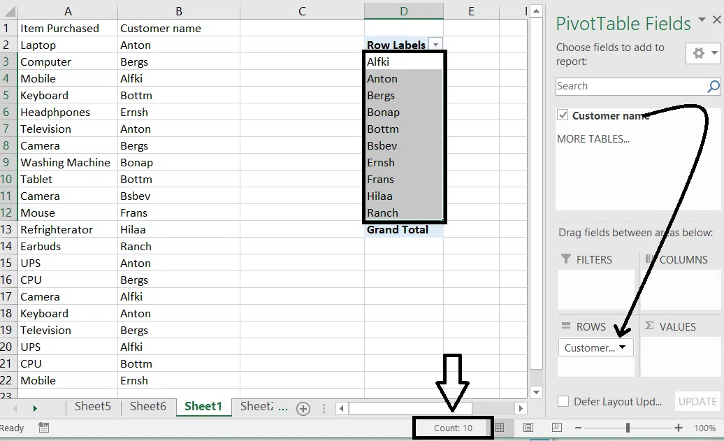
Method 3: Using PivotTables
Pivot Tables are one of Excel’s most powerful tools for summarizing and analyzing data. They also allow you to count distinct values easily. Here's how to do it step-by-step:
Step 1: Create a Pivot Table of the Data
You first need to create a pivot table of Data in which you need to count the Distinct values.
Step 2: Add Data to Rows
- Drag the field (e.g., "Customer Name") you want to analyze into the Rows area of the Pivot Table.
- This will display unique entries for that field as row labels.
Step 3: Add Field to Values and Change to Distinct Count
- Drag the same field into the Values area of the Pivot Table.
- In the Pivot Table field list, click the dropdown next to the field in the Values area and select Value Field Settings.
- In the dialog box, choose Distinct Count and click OK.
Step 4: View the Distinct Count
- The Pivot Table will now display the distinct count of the selected field in the Values are
Method 4: Using Advanced Filters
Advanced filters are a feature in Excel that allows you to specify complex criteria using formulas.
To use advanced filters in Excel, User needs to go to the " DATA" tab, select the "Advanced Filter" option and define the range criteria range and the output range.
This can also help you to find Distinct values in Excel.
Subtotal is the function that can be used to count only the visible items in your list. As shown in the below image, Here 103 argument is used to tell the SUBTOTAL function to Count all the visible items in the particular range.
.png) Enter the Data into the Sheet
Enter the Data into the SheetStep 1: Apply the Filter
- Select your data range and go to Data > Advanced.
- In the dialog box, choose Filter the List, in place and check Unique Records Only.

Step 2: Count Unique Values
- Use the SUBTOTAL Function to count the extracted values.
- You can now see the count of Unique Values in the Range.
.png)
Benefits:
- No formulas required.
- Extracts and displays the unique values for reference
Method 5: Using VBA Macros
For more advanced users, you can use VBA (Visual Basic for Applications) to count unique values. Here’s how to create a custom VBA function. Follow the steps to Count distinct values using VBA:
Step 1: Open the VBA Editor
- Select the Developer Tab in the Excel ribbon.
- If the Developer Tab is not enabled, go to File > Options > Customize Ribbon and enable it.
- Click on Visual Basic in the Developer Tab.
- In the VBA editor, click Insert > Module to open a blank module.
Step 2: Write the VBA Code
Paste the following code into the module:
Function CountUnique(rng As Range) As Long
    Dim Cell As Range
    Dim UniqueValues As Collection
    On Error Resume Next
    Set UniqueValues = New Collection

    For Each Cell In rng
        If Cell.Value <> "" Then
            UniqueValues.Add Cell.Value, CStr(Cell.Value)
        End If
    Next Cell
    On Error GoTo 0

    CountUnique = UniqueValues.Count
End Function
Step 3: Save and Close VBA
- Press Ctrl + S to save your workbook as a Macro-Enabled Workbook (
.xlsm). - Close the VBA editor by pressing Alt + Q.
Step 4: Use the Custom Function
- In Excel, use the function
=CountUnique(range) to count unique values.- Replace
range with the cell range you want to evaluate (e.g., =CountUnique(A1:A10)).
Step 5: Preview the Results
- The function will count unique values in the specified range, ignoring blanks.
This custom VBA function allows you to count unique values easily, just like built-in Excel functions. Save the macro-enabled workbook to preserve the functionality.
Also Read: Countif Function in Excel
How to Count Unique Text or Numeric Values in Excel
Counting unique values in Excel, whether text or numeric, helps you manage datasets effectively by identifying values that appear only once. Below are different methods to achieve this for text, numeric, and case-sensitive values:
Method 1: Counting Unique Text Values
If your dataset in Excel contains both text and numerical values, and you need to count only the unique text values, you can achieve this by combining theISTEXT function with COUNTIF in an array formula. Here's how:
The formula to count unique text values is:
=SUM(IF(ISTEXT(A2:A10)*COUNTIF(A2:A10, A2:A10)=1, 1, 0))
ISTEXT functions return TRUE if the checked value is text value or else FALSE. Here in the formula (*) asterisk works as the AND operator in the formula, which means the IF function returns 1 only if a value is both text and unique, Otherwise 0. And the SUM function adds up all 1's and you can get the count of text values as the output.
Note: Always remember to press Ctrl + Shift + Enter for an array formula.
- Select a blank cell where you want the result to appear.
- Type the formula:
=SUM(IF(ISTEXT(A2:A10)*COUNTIF(A2:A10, A2:A10)=1, 1, 0))
Replace A2:A10 with the actual range of your data.
Step 2: Press Ctrl + Shift + Enter
- For older versions of Excel, press Ctrl + Shift + Enter after typing the formula.
- Curly braces {} will appear around the formula, indicating it is an array formula.
Step 3: View the Result
The formula will return the count of unique text values.
.png) Use the Formula and Preview Results
Use the Formula and Preview ResultsAs you can see the formula returns the value 2, because we have only two text +unique values.
Method 2: Counting Unique Numeric Values
If your Excel list contains both numeric and text values, and you need to count unique numeric values, you can use the ISNUMBER function in combination with COUNTIF. This ensures that only numeric values are considered, excluding text and duplicates.
To count unique numeric values, use the following formula:
=SUM(IF(ISNUMBER(A2:A10)*COUNTIF(A2:A10, A2:A10)=1, 1, 0))
Select a blank cell where you want the result.
=SUM(IF(ISNUMBER(A2:A10)*COUNTIF(A2:A10, A2:A10)=1, 1, 0))
- Replace A2:A10 with the actual range of your data.
- Press Ctrl + Shift + Enter instead of just Enter.
- Curly braces {} will appear around the formula, indicating it is an array formula.
Step 4: View the Result
The formula will return the count of numeric values that appear only once.
.png) Enter the Formula
Enter the FormulaCount Case - Sensitive Unique Values in Excel
The simple way to count unique values when you have Case-Sensitive data would be creating a helper column with the following array formula to identify duplicates and unique items.
If your data is case-sensitive (e.g., "ABC" and "abc" should be considered different), you need to create a helper column and use the following formulas:
Step 1: Create a Helper Column
In the helper column (e.g., Column B), use this formula to identify duplicates and unique values:
=IF(SUM(--EXACT($A$2:$A$10, A2))=1, "Unique", "Duplicate")
- Replace
$A$2:$A$10 with the range of your data. - The
EXACT function performs a case-sensitive comparison. SUM(--EXACT(...)) ensures that only exact matches are considered.
Step 2: Count Unique Values
Use the COUNTIF function to count the number of "Unique" values in the helper column:
=COUNTIF(B2:B10, "Unique")
- Replace
B2:B10 with the range of your helper column.
.png)
In the above image, you can see the Count of unique values is 5.
The COUNTIFS function can be used to count unique values in older versions of Excel. This method leverages an array formula, making it compatible with Excel versions that don’t support dynamic arrays like Excel 365 or 2021.
The formula used is:
=SUM(1/COUNTIFS(B2:B22, B2:B22))
COUNTIFS(B2:B22, B2:B22): This calculates the count of each value in the range B2:B22.1/COUNTIFS(...): Converts the count into fractions, where unique values result in 1, and duplicate values are represented as smaller fractions.SUM(...): Adds up all the results, providing the count of unique values.
- Select a blank cell where you want the result to appear.
- Type the formula
=SUM(1/COUNTIFS(B2:B22, B2:B22))
- Replace
B2:B22 with the range of your data.
For older Excel versions:
- Press Ctrl + Shift + Enter instead of just pressing Enter.
- The formula will automatically be enclosed in curly braces
{}, indicating it’s an array formula
{=SUM(1/COUNTIFS(B2:B22, B2:B22))}
Step 4: View the Result
- The formula will return the count of unique values in the range.

Note: Don't Forget to press the "CTRL+SHIFT+ENTER" to put curly brackets to use an Array formula. Because the array formula doesn't work in older versions of Excel.
Best Practices for Counting Unique Values
- Check for Duplicates: Ensure there are no unintended spaces, formatting issues, or invisible characters that may affect results.
- Use Dynamic Ranges: When working with datasets that change frequently, use structured references or dynamic ranges.
- Combine Methods: Use a combination of
UNIQUE, pivot tables, and Power Query for maximum flexibility.
Common Issues and Troubleshooting
- Hidden Duplicates: Use the TRIM function to remove extra spaces before counting unique values.
- Incorrect Ranges: Double-check your formulas to ensure the correct range is referenced.
- Formula Errors: For array formulas, always press Ctrl + Shift + Enter to activate them properly in older Excel versions.
Conclusion
Mastering the ability to count unique Excel values is an essential skill for anyone working with data. By using techniques like the UNIQUE function, COUNTIF formulas, or the Excel count distinct values feature, you can streamline your workflow and ensure accurate reporting. Utilizing a count distinct Excel pivot table setup allows you to handle large datasets dynamically, while formulas offer precision for targeted calculations. No matter the method, understanding these tools will help you confidently manage and analyze data. Apply these skills to tasks like tracking sales, managing inventory, or generating professional reports to improve efficiency and accuracy in your work.
Similar Reads
How to Count Distinct Values in MySQL?
The COUNT DISTINCT function is used to count the number of unique rows in specified columns. In simple words, this method is used to count distinct or unique values in a particular column. In this article, we are going to learn how we can use the Count Distinct function in different types of scenari
5 min read
How to Count Distinct Values in PL/SQL?
PL/SQL, an extension of SQL for Oracle databases, allows developers to blend procedural constructs like conditions and loops with the power of SQL. It supports exception handling for runtime errors and enables the declaration of variables, constants, procedures, functions, packages, triggers, and mo
5 min read
Splitting Cells and Counting Unique Values in Python List
Here, we need to split elements of a list and count the unique values from the resulting segments. For example, given a list like ["a,b,c", "b,c,d" , e,f"], we want to extract each value, count only the unique ones, and return the result. Let’s examine different methods to achieve this, starting fro
3 min read
How to Find Unique Values and Sort Them in R
Finding and Sorting unique values is a common task in R for data cleaning, exploration, and analysis. In this article, we will explore different methods to find unique values and sort them in R Programming Language. Using sort() with unique()In this approach, we use the unique() function to find uni
2 min read
How to Sum Values Based on Criteria in Another Column in Excel?
In Excel, we can approach the problem in two ways. [SUMIF Formula and Excel Pivot] Sample data: Sales Report Template We are creating a summary table for Total Product sales. Approach 1: Excel Formula SUMIF Step 1: Copy “Column A†Products and then paste into “Column F†Step 2: Remove duplicate prod
1 min read
How to count unique values in a Pandas Groupby object?
Here, we can count the unique values in Pandas groupby object using different methods. This article depicts how the count of unique values of some attribute in a data frame can be retrieved using Pandas. Method 1: Count unique values using nunique() The Pandas dataframe.nunique() function returns a
2 min read
How to Find Duplicate Values in Excel Using VLOOKUP?
In this article, we will look into how we can use the VLOOKUP to find duplicate values in Excel. To do so follow the below steps: Let's make two columns of different section to check VLOOKUP formula on columns:Created Two Columns Here is the formula we are going to use:=VLOOKUP(List1,List2,TRUE,FALS
2 min read
How to Create a Contingency Table in Excel
A contingency table, also known as a crosstab is used to show the relationship between two categorical variables. In Excel, we can make a contingency table using the pivot table function. They are best for summarizing the relationship between categorical variables. A contingency table is just like a
4 min read
Get unique values from a column in Pandas DataFrame
In Pandas, retrieving unique values from DataFrame is used for analyzing categorical data or identifying duplicates. Let's learn how to get unique values from a column in Pandas DataFrame. Get the Unique Values of Pandas using unique()The.unique()method returns a NumPy array. It is useful for identi
5 min read
How to Count Words in Excel
Excel is a tool for storing, organizing, and visualizing a large volume of data. It uses a rectangular block known as a cell to store the data unit. This tool can be used to perform different tasks like creating graphs and analyzing trends, to get insights from the data. Data analysis can be perform
6 min read