How to Calculate Average in Excel: Essential Formulas & Examples for 2024

Whether you’re a student crunching numbers for a project, a business analyst examining sales data, or simply someone looking to get insights from personal data, mastering the art of calculating averages in Excel can significantly enhance your data-handling capabilities.

In this article, you will learn the basic average functions in Excel along with examples and even touch on some tricks for handling more specific needs.

Why Calculate Averages

Calculating averages is essential for summarizing large sets of data, identifying trends, and making informed decisions. In Excel, there are several functions to help you find averages, each suited to different scenarios. Let’s explore the most commonly used methods and functions.

How To Calculate Average Manually in Excel

To calculate the average without using the AVERAGE function, we can sum all numeric values and divide by the count of numeric values. We can use SUM and COUNT functions like this:

= SUM(A1:A5)/COUNT(A1:A5)            // manual average calculation

Here:

• SUM function is used to add multiple numeric values within different cells and
• COUNT function to count the total number of cells containing only numbers.

Let us look at an example :

Here we are calculating the average age of all the customers from Row 2 to Row 12 using the formula :

SUM(B2:B6)/COUNT(B2:B12) 

Excel AVERAGE function

To calculate the average (or mean) of the given arguments, we use the excel function average. In AVERAGE ,maximum 255 individual arguments can be given and the arguments  which can include numbers / cell references/ ranges/ arrays or constants.

Syntax :
= AVERAGE(number1, [number2], ...)

• Number1 (Required) : It specifies the Range, cell references or first number for which we want the average to be calculated.
• Number2 (Optional) : Numbers, cell references or ranges which are additional for which you want the average.

For example: If the range C1:C35 contains numbers, and we want to get the average of those numbers, then the formula  is : AVERAGE(C1:C35)

Note:

1. Those values in a range or cell reference argument which has text, logical values, or empty cells, are ignored in calculating average.
2. Cells with the value zero are included.
3. Error occur if the arguments have an error value or text that cannot be translated into numbers.

Let us look at the same example to calculate the average age of all the customers  from row 2 to row 12 using the formula : AVERAGE(B2:B12).

If we have a row containing non-numeric value, it is ignored as :

Here average of rows from B2 to B6 was taken, but B5 is not included in the average as it contain non numeric data.

You can see that in column B : we have done B7 = AVERAGE (B2 : B6) .

So AVERAGE() will evaluate as = 9+8+8+9 / 4 = 8.5

Excel AVERAGEA Function

To calculate the average (or mean) of all the non-blank cells, we use the Excel function AVERAGEA. The AVERAGEA function is not same as the AVERAGE function, it is different as AVERAGEA treats TRUE as a value of 1 and FALSE as a value of 0.

The AVERAGEA function was introduced in MS Excel 2007( Not in old versions) & it is a statistics related function.

It finds an average of cells with any data (numbers, Boolean and text values) whereas the average()  find an average of cells with numbers only.

Syntax:
=AVERAGEA(value1, [value2], …)

Value1 is required, subsequent values are optional. 

In AVERAGEA ,up to 255 individual arguments can be given & the arguments  which can include numbers / cell references/ ranges/ arrays or constants.

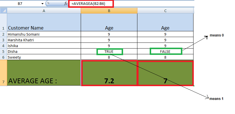
Here , you can see that :

1. In column B : we have done B7 = AVERAGEA(B2 : B6). So AVERAGEA() will evaluate as = 9+9+9+1+8 / 5 = 7.2 (True is replaced by 1 in calculating).
2. In column C : we have done C7 = AVERAGEA(C2 : C6) .

So AVERAGEA() will evaluate as = 9+9+9+0+8 / 5 = 7 (False is replaced by 0 in calculating)

Note: AVERAGE just skips these values (true/false) during calculation. So, if you do not want to include logical values (True/False), use the AVERAGE function.

Excel AVERAGEIF Function

To calculate the average (or mean) of the given arguments that meet a (single) given criteria, we use the Excel function AVERAGEIF.

Syntax :
= AVERAGEIF(range, criteria, [average_range])

Here :

• Range : Required, It specifies the range of cells that needs to be tested against the given criteria.
• Criteria : Required , the condition used to determine which cells to average. The criteria specified here can be in the form of a number,  text value, logical expression, or cell reference, e.g. 5 or “>5” or “cat” or A2.
• Average_range : Optional , The set of cells on which the average needs to be calculated on. If not included , the range is used to calculate the average on.

Note :

1. AVERAGEIF ignores an empty cell in average_range.
2. AVERAGEIF ignores Cells in range that contain TRUE or FALSE.
3. AVERAGEIF returns the #DIV0! error value, if range is a blank or text value
4. AVERAGEIF treats cell value as a 0 value, If a cell in criteria is empty.

Example 1: Let us look at an example that calculate average of non negative ages of customers in the rows 2 to 6 :

Here : The negative age is not included in the average. Average is calculated as = (9+8+9+9) / 4 = 8.75

Example 2: To get the average of price of the product named : “Apple” :

Here in the criteria, we specified “Apple” & in range we specified A2: A6 & we are doing average on B2:B6 (Price), so in the  range A2: A6, wherever Apple comes, include its price for calculating average.

Here, average is calculated as : 100 + 200 / 2 = 150.

Excel AVERAGEIFS Function

To calculate the average (or mean) of the given arguments that meets multiple criteria, AVERAGEIFS is used.

Syntax :
= AVERAGEIFS(average_range, criteria1_range1, criteria1, [criteria2_range2, criteria2], ...)

Here,

• average_range : Required, The range of cells that you wish to average.
• criteria1_range2, criteria2_range2, … criteria1_range2 is required. The range to apply the associated criteria against.
• criteria1, criteria2, … criteria1 is mandatory, further more criteria are optional.

Note : The criteria to apply against the associated range. Criteria1 is the criteria to use on range1 and the criteria2  is the criteria to use on range2 and so on.

Example: To calculate the average price of Product named “Apple” and whose price > 99 :

Here 2 conditions are met :

• 1st condition range – A2:A6 and criteria is “Apple“, 3 rows matches the criteria
• 2nd Condition range – B2:B6 and criteria is  “>99” & there are 3 rows with product name apple & with price >99

So, the average is = (100 + 120 + 200) / 3 = 140

Average Cells by Multiple Criteria with OR Logic

This logic test multiple conditions at the same time. OR returns either TRUE or FALSE. For example, to test A1 contains “x” or “y”, use =OR (A1=”x”, A1=”y”).

Example: To see that the product in a particular row is an apple/ an orange , we can :

Here we can see that the product in the range A2 to A6 having name : Apple / orange evaluates true result in the column B2 to B6. Now we can use this sub-result as a part of our function AVERAGEIFS().

Example: To calculate the average price of the product named Apple/ Orange having price > 99 :

We use the method as : 

=AVERAGEIFS(C2:C6,B2:B6,"True",C2:C6,">99")

As you can see that to add OR with the AVERAGEIFS() , we add a new column that takes the result of the OR query , i.e., either true/false . Based on that answer , we are calculating the average by matching True for the range B2:B6.

So the average comes out to be 

= (100 + 120 + 200) / 3 = 140.

We considered only those price which were > 99 for the product : Apple / Orange.

Conclusion

Calculating averages in Excel is a fundamental skill for anyone working with data. Whether you use basic functions like SUM and COUNT or more advanced functions like AVERAGEIFS, mastering these techniques will enable you to analyze and summarize your data effectively. By understanding and applying these methods, you can enhance your data analysis capabilities and make better, data-driven decisions.