Hierarchies in Excel Power Pivot

Last Updated : 29 Dec, 2022

A Hierarchy is a system that has many levels from highest to lowest. When we have related columns in a table, then analyzing them with fixed attributes is difficult. Excel Power Pivot gives us the power to set a hierarchy to which data can be filtered and analyzed correctly according to one's needs. In this article, we will learn how to create hierarchies in the Power pivot.

Meaning of Hierarchy in Power Pivot

Hierarchy in a data set helps analyze complex data easily. A hierarchy is a list of nested columns in a table. Power Pivot hierarchies provide additional features and functionalities to help classify and analyze data efficiently. Hierarchy helps provide a large amount of data in a space-efficient manner. Power pivot hierarchies have aggregate functions like Count, Min, Max, Average, and Distinct Count, which help analyze different aspects of the data. One can also move to different levels in the hierarchy by the drill up and drill down option provided by PivotTableAnalyze. For example, Department, Project, and Employee all three columns can be combined into a single column as a hierarchy.

Creating a Hierarchy By Power Pivot

Given a data set, with a table in an excel sheet name Employee. The Attributes of the table are Employee Id, Employee Name, Department, and Salary. We need to create a hierarchy of Department ⇢ Employee Name providing Salary as values. Save the given excel sheet with employee.xlsx.

Step 1: Open a new blank sheet. Go to Power Pivot, and click on Manage.

Step 2: A new window name Power Pivot for Excel is opened.

Step 3: Go to the Home tab. Under the Get External Data section, click on From Other Sources.

Step 4: A new window name Table import Wizard is opened. Under Text Files. Select Excel Files option. Click on Next.

Step 5: Firstly, check the box, Use First Row as column headers. Then, click on Browse.

Step 6: Select the file employee.xlsx. Click on Ok.

Step 7: The desired file is selected. Click on the Next button.

Step 8: Select the tables that you want to add to your power pivot. Click on the Finish button.

Step 9: The files will be imported and a success pane will appear. Click on the Close button.

Step 10: Power Pivot window reappears. A table is inserted in your Power Pivot.

Step 11: Now, go to the Home tab. Under the view section, click on the Diagram View.

Step 12: The diagram view of the table appears with the names of the attributes.

Step 13: Select the attributes you want in your hierarchy. For example, Department. The order in which you select the hierarchy is important, as the attribute selected first will appear at a higher level than the later selected attribute.

Step 14: To select multiple attributes, press Ctrl + mouse click.

Step 15: After selecting the desired attributes. Right-click on the Create Hierarchy.

Step 16: A new attribute is created. Rename the attribute to your choice. For example, renaming the new attribute to Hierarchy.

Step 17: Go to the Home tab. Select PivotTable.

Step 18: A Create PivotTable dialogue box appears. Select the radio button, new worksheet, and click on Ok.

Step 19: PivotTable Fields appear on the right-most side of the worksheet.

Step 20: Drag and Drop Hierarchy to Rows. A table with the highest level hierarchy appears.

Step 21: Drag and Drop Salary to Values.

Step 22: A Hierarchy table is created. You can click on the + button, to move down to the next level in the hierarchy.

Exploring Different Features in Power Pivot Hierarchy

Now, we will explore different features in the hierarchy offered by the power pivot. Consider the hierarchy created above. i.e. Department ⇢ Employee Name.

Changing the order in a Hierarchy

Given the Drawing View of the Employee Table.

Use Move Up and Move Down buttons to change the order of your hierarchy.

Step 1: Select any attribute in the hierarchy. For example, Department. Right-click on it.

Step 2: Click on the Move Down button.

Step 3: This moves your attribute in the hierarchy to one level down. For example, the Department attribute comes under the Employee Name now.

Step 4: Again, Right-click on the Department. Click on the Move Up button.

Step 5: The Move Up button moves your attribute to one level up in the hierarchy. For example, the Employee Name attribute comes under the Department now.

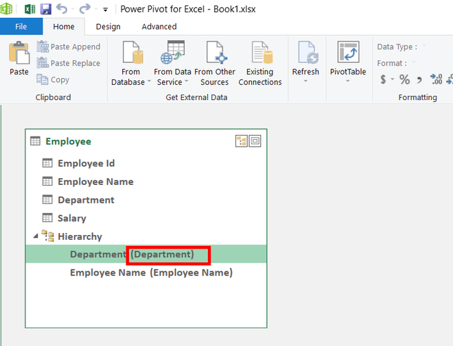
Hiding or Showing Source column name in the Hierarchy

Given the Drawing View of the Employee table.

The Source Column Name can be different from the name in the Hierarchy.

Step 1: The text written in the Parenthesis is the Source Column Name. By default, the Source Column Name and the Hierarchy Column Name are the same.

Step 2: Right-Click on any attribute of the hierarchy attribute. Click on the Hide Source Column Name.

Step 3: The text is written in the parenthesis disappears.

Drill Up and Drill Down in the Hierarchy

Consider the Hierarchical Pivot table created above.

Drill Up and Drill down are used to come down or up a level in the hierarchy.

Step 1: Select cell B6 in the hierarchical pivot table. The department is IT.

Step 2: Go to the PivotTable Analyze tab. Click on the Drill Down button.

Step 3: Now, the name of the employees will appear, working in that department. The selected cell moves down to one level.

Step 4: To Drill Up in the table. Select any cell in the Hierarchy attribute. For example, select cell B4 i.e. Arushi.

Step 5: Click on the Drill Up button.

Step 6: The table reaches back to its previous level.

Create An Hierarchy using In related Tables

Creating Hierarchy between multiple tables is not possible in Power pivot. To add attributes of another table in your parent table can only be achieved if you add that attribute from another table to your parent table. Given a data set of two tables, one named Employee and the second named Project in two different excel sheets in the same workbook. For example, create a hierarchy of Department ⇢ Project Id ⇢ Employee Name. As Project Id is not present in the Employee table so we will add the Project Id attribute from the Project table to the Employee table.

Step 1: Create a Drawing view, of both the tables in the power pivot window, by importing the file in the power pivot window.

Step 2: Now, create a relation between the Employee table and the Project table. To do this, there should be at least one attribute common in both of the tables. Keep your cursor on the Employee table, select any attribute and drag the mouse to the Project table, leave your mouse click.

Step 3: A small arrow line is created between the tables, showing that both tables are related.

Step 4: Go to the Home tab, and click on the Data view option.

Step 5: Click on the Add Column.

Step 6: Write a function =RELATED([Project Id]) in the ribbon. Press Enter.

Step 7: A column name Calculated Column 1 is added to the Employee table.

Step 8: Rename the attribute as Project Id.

Step 9: Go to the Home tab, and click on the Draw View. Select the Attributes in the hierarchical order to be created i.e. Department ⇢ Project Id ⇢ Employee Name. Click on the Create Hierarchy.