Goal Seek in Excel is a What-If Analysis tool that finds the input value needed to achieve a specific result in a formula. It automatically adjusts one variable to reach the desired output, making it useful for calculations like savings targets, interest rates, or totals.
1. Using Goal Seek
Goal Seek in Excel adjusts an input value to achieve a specific target in a formula. Simply set the desired result, and Excel calculates the required input automatically. Follow the below steps to learn how to use Goal Seek in Excel:
Step 1: Set Up Your Data
- Enter your formula in a cell.
- Make sure the formula cell reflects the result you want to manipulate.
In the below example, You want to save $10,000 in 24 months, and you want to calculate how much you need to save each month to meet this goal.

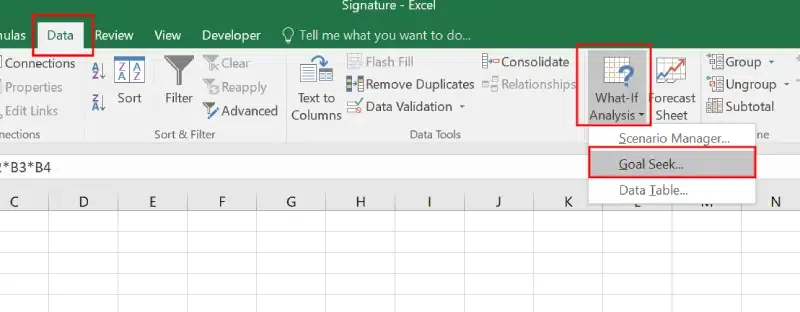
Step 2: Open Goal Seek
- Go to the Data tab in the Ribbon.
- Click What-If Analysis and select Goal Seek from the dropdown
Pro Tip: Use Alt + A, followed by W, and then G as a shortcut to open Goal Seek quickly.

Step 3: Fill Out the Goal Seek Dialog Box
- Set Cell: Select the cell that contains the formula.
- To Value: Enter the target value you want to achieve.
- By Changing Cell: Select the cell that Excel should adjust to reach the target.

Step 4: Run Goal Seek and Review Results
Click OK, and Excel will calculate the necessary input value. The adjusted input will appear in the selected cell. Verify the solution to ensure it meets your needs, and if needed, adjust your data or formula and run Goal Seek again.
Note: Goal seek works with only one variable input at given time. You can use the Solver in Excel for multiple input values.

2. Excel Goal Seek Examples
Here are some practical Excel Goal Seek examples to help you understand how to use this tool for solving real-world problems.
Example 1: Calculating the Rate of Interest
Scenario: You need to calculate the rate of interest when the principal amount, time period, and simple interest are already known.
Given Data:
| Principal | Time | Simple Interest | Rate |
|---|---|---|---|
| $2,000 | 3 years | $6,000 | ? |
Step 1: Enter the Data
Open Excel and enter the given values (e.g., Principal in B2, Time in B3, Simple Interest in B5).

Step 2: Write the formula
In B5, write the formula for Simple Interest.
=B2 * B3 * B4
- B4 will be the rate of interest we need to calculate.

Step 3: Open Goal Seek
Go to the Data tab, select What-If Analysis, and click Goal Seek.
Step 4: Set the Parameters
- Set cell: Select the cell containing the Simple Interest formula (B5).
- To value: Enter 6000 (the desired result).
- By changing cell: Select the cell where the interest rate is calculated (B4).

Step 5: Run Goal Seek and Preview the Result
Click OK, and Excel will calculate the interest rate. The result will be displayed in cell B4 for your review.

Things to Remember:
- The Set Cell must contain a formula.
- There must be a dependency between the Set Cell and the Changing Cell.
- Avoid using special characters or invalid entries in the Changing Cell.
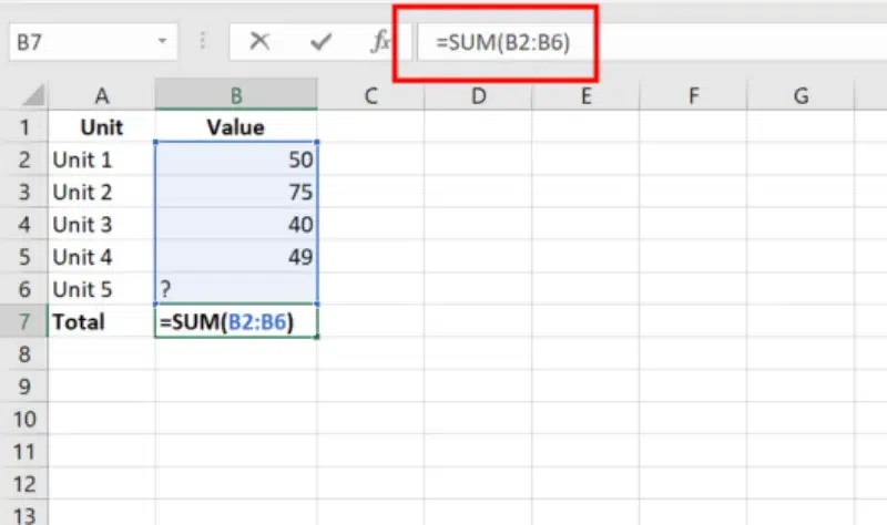
Example 2: Determining a Missing Value to Achieve a Target Total
Scenario: Calculate a missing value so that the sum equals 303.
Step 1: Enter the Values
Input the known values in separate cells and leave the missing value cell blank.

Step 2: Write the SUM Formula
In a cell (e.g., B7), write the formula to calculate the total.
=SUM(B2:B6)
Step 3: Open Goal Seek
Click on theData tab, select What-If Analysis, and choose Goal Seek.
Step 4: Set the Parameters
- Set cell: Select the cell containing the SUM formula (e.g., B7).
- To value: Enter 303 (the desired total).
- By changing cell: Select the blank cell where the missing value will go (e.g., B6).

Step 5: Run Goal Seek
Click OK to calculate the missing value.
Step 6: Preview the Result
Excel will calculate and display the missing value (e.g., 89 for Unit 5).

Example 3: Finding Missing Marks for a Student’s Average
Scenario: You need to calculate the marks required in a specific subject for a student to achieve a final average of 83.
Step 1: Enter the Data
Input the student’s marks for other subjects in separate cells and leave the missing subject cell blank.

Step 2: Write the Average Formula
In a cell (e.g., B7), write the formula to calculate the average:
=AVERAGE(B2:B6)
Step 3: Open Goal Seek
Go to the Data tab, click on What-If Analysis, and select Goal Seek.
Step 4: Set the Parameters
- Set cell: Select the cell containing the formula for the average (e.g., B7).
- To value: Enter 83 (the desired average).
- By changing cell: Select the blank cell for the missing subject’s marks (e.g., B6).

Step 5: Run Goal Seek
Click OK to calculate the required marks.
Step 6: Preview the Result
Excel will display the required marks in B6 (e.g., 74).
