How to Apply Conditional Formatting Based On VLookup in Excel?

VLOOKUP is an Excel function to lookup data in a table organized vertically. VLOOKUP supports approximate and exact matching, and wildcards (* ?) for partial matches.

Conditional Formatting Based on Vlookup:

1. Using the Vlookup formula to compare values in 2 different tables and highlighting those values which is only present in table 1 using conditional formatting. 

We have a Table containing old products of any grocery shop in 'Old Product' sheet and an updated table having new products in worksheet 'New'. We want to highlight rows in New table containing those items which are not in Old Product Table.

• Select the data from New table except the Headers. (The table in which we want to highlight rows.)

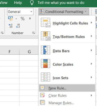
• Go to Home->Conditional Formatting->New Rule.

• In the dialog box appeared, Select the rule type - "Use a formula to determine which cells to format;";
• Under Edit the rule description enters the following formula:

 =ISNA(VLOOKUP($A2,'Old Product'!$A$1:$B$8,1,FALSE))

• Then click Format.

Formula explanation:

Inside VLOOKUP, 

• 1st parameter is $A2 which is first name in New table.
• 2nd parameter is Old Product Table.
• 3rd parameter is column we want to compare which is 1 as we want to compare item names.
• 4rd parameter is False i.e. only exact values are matched.

So, this formula will return a valid value for those New Table items which are found in Old Table and #NA for those which are not found. 

Now, if the value is NA we want to Highlight them as they are not in old product table. So, they are new items added. Using ISNA we will achieve this. 

Finally, we have the required values and we will highlight them.

• A new dialog box will appear. Go to Fill Tab and select a color to fill.

• Click OK to close both the dialog boxes.
• Now, Those value which is present in New table but not in Old Product will be highlighted.

 2. Using the Vlookup formula to compare values in 2 different tables and highlighting those values which is greater in table 1 as compared to table 2 using conditional formatting.

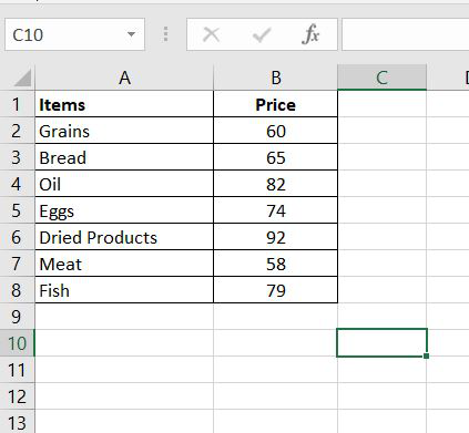
We have a Table containing the old price of some grocery items in the 'Old Product' sheet and a table having a new price of those grocery items in the worksheet 'New'. We will highlight those rows in the Old Product Table in which a particular item's cost is greater than that of the New table.

• Select the data from the old price table except for the Headers.

• Go to Home->Conditional Formatting->New Rule.

• In the dialog box that appeared, Select the rule type - "Use a formula to determine which cells to format;"
• Under Edit the rule description enter the following formula 

 =(VLOOKUP($A2, 'New'!$A$1:$B$8,2,FALSE)<'Old Product'!$B2 

• And click Format.

Formula explanation:

Inside VLOOKUP,

• 1st parameter is $A2 which is first name in Old Product table.
• 2nd parameter is New Table.
• 3rd parameter is column we want to compare which is 2 in New Table as we want to compare Price.
• 4rd parameter is False i.e. only exact values are matched.

Now we will compare this with cost value in Old Product table starting from 1st value. If cost is greater than we will highlight.

• A new dialog box will appear. Go to Fill Tab and select a color to fill.

• Click OK to close both the dialog boxes.

This is how we can apply conditional formatting based on VLookup.