How to Add a Calculated Field to a Pivot Table in Excel
Last Updated :
23 Dec, 2024
A Calculated Field in Pivot Table allows you to perform custom calculations within your Excel Pivot Table, giving you more flexibility and deeper insights into your data. Whether you need to add a custom formula, modify existing calculations, or remove a field, this guide walks you through the essential steps. By learning how to add a calculated field to a Pivot Table, you'll unlock the potential for advanced data analysis and customization, helping you make informed decisions with ease.
How to Add a Calculated Field to a Pivot Table
Adding a calculated field lets you apply a custom formula directly within your Pivot Table to analyze data more effectively. Here’s how to add a calculated field to a Pivot Table:
Step 1: Open the Pivot Table
- Open the Excel workbook that contains your Pivot Table.
- Ensure the Pivot Table is created and the data fields you want to use for calculations are present.
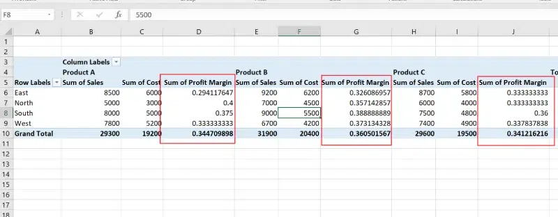
The image below summarizes the sales and cost data by region (row labels) and product (Column labels). The Pivot Table includes the following fields:
- Columns: Products (Product A, Product B, Product C) with their respective "Sum of Sales" and "Sum of Cost."
- Rows: Regions (East, North, South, West), showing totals for each region across all products.
- Values: The sum of sales and costs for each product in each region, along with the grand totals for sales and costs at the bottom.
- The Pivot Table Fields panel is visible on the right, displaying the fields used: Region (Rows), Sales, and Cost (Values), and Product (Columns). This setup allows for a clear analysis of sales and costs by product and region.
 Pivot Table
 Step 2: Access the Calculated Field Option
- Click anywhere inside the Pivot Table to activate the PivotTable Analyze tab on the ribbon.
- Go to PivotTable Analyze (or Options in older versions of Excel).
- In the Calculations group, click Fields, Items & Sets, and then select Calculated Field.
 Go to Analyze Tab>>Fields, Items and Sets >> Select Calculated Field
Step 3: Create a New Calculated Field
In the Insert Calculated Field dialog box that appears
Enter a name for your calculated field in the Name box (e.g., "Profit Margin")
Write the formula for the calculation in the Formula box using the available fields.
- Use the Field list to select fields and click Insert Field to include them in the formula.
- For example: To calculate "Profit Margin" as (Sales - Cost) / Sales, write:
=(Sales-Revenue)/ Sales
Click OK to add the calculated field.
 Enter a Name for your Field >>Enter Formula >> click ok
Step 4: Preview the Calculated Field
- The new calculated field will appear as a column or row in the Pivot Table based on your layout.
- Excel will automatically perform the calculation for all data points in the Pivot Table.
 Preview the Calculated Field
How to Modify a Calculated Field in Pivot Table
If you need to update or adjust a calculated field, follow these steps to modify a calculated field in Excel:
- Click anywhere inside the Pivot Table.
- Go to PivotTable Analyze > Fields, Items & Sets > Calculated Field.
- In the dialog box, select the calculated field from the Name dropdown.
- Modify the formula and click OK
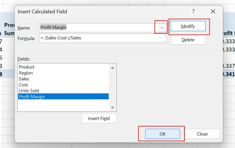 Click on the Calculated Field Name Drop-Down >> Click on Modify>> Modify the Formula >> Click ok
How to Delete a Calculated Field in Pivot Table
If you need to delete a calculated field in Excel, follow these simple steps:
Step 1: Access the Calculated Field Option
Click anywhere inside the Pivot Table. Go to the PivotTable Analyze tab on the ribbon and then Click Fields, Items & Sets, and select Calculated Field.
 Go to Analyze Option >>Select "Fields, Items & Sets" >> Click on Calculated Field
Step 2: Select the Field to Delete and Click on Delete
- In the Insert Calculated Field dialog box, open the Name dropdown.
- Select the calculated field you want to delete.
- Click the Delete button in the dialog box and Confirm by clicking OK.
 Click on the Drop-Down>>Select the Calculated Field>>Press Delete>> Click OK
Step 3: Preview Result
The calculated field will be removed from the Pivot Table.
 Calculated Field have been removed
Also Read:
Conclusion
Mastering the use of a Calculated Field in Pivot Table enhances your ability to perform dynamic calculations directly within your data analysis. Whether you want to add a calculated field to a Pivot Table, modify it for evolving needs, or delete a calculated field in Excel, these steps equip you with the skills to manage data effectively. Incorporate these Excel Pivot Table advanced tips to streamline your reporting process and achieve greater accuracy in your analysis.
Similar Reads
Non-linear Components In electrical circuits, Non-linear Components are electronic devices that need an external power source to operate actively. Non-Linear Components are those that are changed with respect to the voltage and current. Elements that do not follow ohm's law are called Non-linear Components. Non-linear Co
11 min read
Spring Boot Tutorial Spring Boot is a Java framework that makes it easier to create and run Java applications. It simplifies the configuration and setup process, allowing developers to focus more on writing code for their applications. This Spring Boot Tutorial is a comprehensive guide that covers both basic and advance
10 min read
Class Diagram | Unified Modeling Language (UML) A UML class diagram is a visual tool that represents the structure of a system by showing its classes, attributes, methods, and the relationships between them. It helps everyone involved in a project—like developers and designers—understand how the system is organized and how its components interact
12 min read
Backpropagation in Neural Network Back Propagation is also known as "Backward Propagation of Errors" is a method used to train neural network . Its goal is to reduce the difference between the model’s predicted output and the actual output by adjusting the weights and biases in the network.It works iteratively to adjust weights and
9 min read
3-Phase Inverter An inverter is a fundamental electrical device designed primarily for the conversion of direct current into alternating current . This versatile device , also known as a variable frequency drive , plays a vital role in a wide range of applications , including variable frequency drives and high power
13 min read
Polymorphism in Java Polymorphism in Java is one of the core concepts in object-oriented programming (OOP) that allows objects to behave differently based on their specific class type. The word polymorphism means having many forms, and it comes from the Greek words poly (many) and morph (forms), this means one entity ca
7 min read
CTE in SQL In SQL, a Common Table Expression (CTE) is an essential tool for simplifying complex queries and making them more readable. By defining temporary result sets that can be referenced multiple times, a CTE in SQL allows developers to break down complicated logic into manageable parts. CTEs help with hi
6 min read
What is Vacuum Circuit Breaker? A vacuum circuit breaker is a type of breaker that utilizes a vacuum as the medium to extinguish electrical arcs. Within this circuit breaker, there is a vacuum interrupter that houses the stationary and mobile contacts in a permanently sealed enclosure. When the contacts are separated in a high vac
13 min read
Python Variables In Python, variables are used to store data that can be referenced and manipulated during program execution. A variable is essentially a name that is assigned to a value. Unlike many other programming languages, Python variables do not require explicit declaration of type. The type of the variable i
6 min read
Spring Boot Interview Questions and Answers Spring Boot is a Java-based framework used to develop stand-alone, production-ready applications with minimal configuration. Introduced by Pivotal in 2014, it simplifies the development of Spring applications by offering embedded servers, auto-configuration, and fast startup. Many top companies, inc
15+ min read