Excel COUNTIF Function for Exact and Partial Match (With Examples)
Last Updated :
17 Dec, 2024
The COUNTIF function in Excel is a powerful tool used to count cells that meet specific criteria, whether it's an exact match or a partial match. This function is incredibly useful for managing large datasets, analyzing trends, or summarizing data quickly. For example, you can use COUNTIF to count how many times a specific word appears in a list or identify cells containing partial matches like text strings.
With its ability to handle both numeric and text-based data, the COUNTIF function simplifies tasks like tracking inventory, analyzing survey responses, or checking for duplicates. In this guide, we’ll break down how to use the COUNTIF function for both exact and partial matches with clear examples and step-by-step instructions.
 Excel COUNTIF Function for Exact and Partial Match
Understanding COUNTIF Function
The COUNTIF function counts the number of cells within a range that satisfy a given condition or "criteria." This makes it ideal for summarizing data or performing quick checks across large datasets. Here’s the syntax of the function:
=COUNTIF(range, criteria)
- range: The range of cells you want to evaluate.
- criteria: The condition that a cell must meet. This can be a number, text, or logical expression. If you're using text, the criteria must be enclosed in quotation marks.
For example, you can use COUNTIF to count how many times a specific word, number, or text string appears in a dataset.
Count Exact Matches with Text in Excel
In many cases, you might want to count how many times a specific word appears in a range, regardless of its position. The COUNTIF function is case-insensitive by default, meaning it will count occurrences of a word regardless of whether it's written in uppercase or lowercase.
Step 1: Prepare your Data
Make sure you have your data in place. In this example, column A contains fruit names.
 Enter Data into excel Sheet
Step 2: Select a Cell for the Result
Click on the cell where you want the result to appear (e.g., B2).
 "B2" Cell Selected
 In the selected cell, enter the following formula:
=COUNTIF(A2:A6, "Apple")
This will count how many times the word "Apple" appears in the range A2:A6.
Here's a breakdown of the formula:
- A2:A6: This is the range where Excel will look for the word "Apple". It refers to cells A2 through A6.
- "Apple": This is the criteria. It tells Excel to count only the cells that contain exactly the word "Apple". The text must match exactly, including capitalization and spacing. If you need to count different variations like "apple" or "APPLE", Excel’s COUNTIF is case-insensitive by default.
 Enter the Formula
 Step 4: Press Enter
After pressing Enter, Excel will return the count. In this case, the result is 3, since "Apple" appears three times in the range.
 Press Enter and Preview Result
 Count Exact Matches with Numbers in Excel
The COUNTIF function can also be used to count exact numeric values. Unlike text, you don’t need quotation marks around numbers.
Example: Let’s say you want to count how many times the number 10 appears in a list of values.
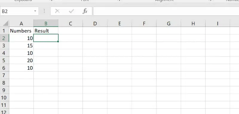
Step 1: Prepare your Data
Enter your numbers in column A.
 Enter data into the Sheet
 Step 2: Select a Cell for the Result
Click the cell where you want the result to appear (e.g., B2).
 Select a Cell to Display Result
 Use the following formula:
=COUNTIF(A2:A6, 10)
A2:A6 refers to the cells within the range A2 to A6 in column A. This is the range of cells in which Excel will search for the number 10.
Step 4: Press Enter
The result will be 3, since the number 10 appears three times in the range.
Counting Cells with Specific Text Using Wildcards
In Excel, wildcard characters allow you to count cells that match specific text patterns, rather than requiring an exact match. These wildcard characters are particularly useful when working with large datasets where the exact text may vary, but the general pattern remains the same.
Here are the two main wildcard characters that can be used with the COUNTIF function:
1. Asterisk (*) - Represents Any Number of Characters
The asterisk (*) wildcard represents any sequence of characters, including no characters at all. This means it can match any part of a text string, allowing you to count cells that contain text, regardless of what comes before or after it.
- Use Case: If you're searching for any cell that contains a certain word or letter within a larger string, you can use the
* wildcard.
Example: How to Count Cells with Partial Text (Using Asterisk)
Let’s say you want to count how many fruit names start with the letter "A".
Step 1: Prepare Your Data
Have your data in place, for example:
| A |
|---|
| Apple |
| Banana |
| Apricot |
| Orange |
| Avocado |
Step 2: Select a Cell for the Result
Click on the cell where you want the result to appear (e.g., B2).
Use the following formula to count cells that start with "A"
=COUNTIF(A2:A6, "A*")
More Use Cases:
"A*": This would match any cell where the text starts with the letter "A" and is followed by any characters (e.g., "Apple", "Avocado", "Apricot")."*berry": This would match any cell where the text ends with "berry" (e.g., "Strawberry", "Blueberry", "Gooseberry")."*apple*": This would match any cell that contains the word "apple" anywhere in the text (e.g., "Green Apple", "Apple Pie", "Pineapple").
Step 4: Press Enter
The result will be 4, since four fruit names start with the letter "A" (Apple, Apricot, Avocado, etc.).
2. Question Mark (?) - Represents a Single Character
The question mark (?) wildcard represents a single character. This is useful when you know the structure of the text but one or more characters might vary. It can be used to match specific text with an unknown or flexible character at a single position.
- Use Case: The
? wildcard is helpful when you know the length and structure of the text, but you're unsure about one specific character.
Example: How to Count Cells with Partial Text (Using the Question Mark Wildcard)
Let’s say you want to count how many names contain "J" as the first character and "n" as the third character (e.g., "Jan", "Jon", "Jen").
=COUNTIF(A2:A10, "J?n")
This formula will count all three-letter names starting with "J" and ending with "n".
Important Notes
- Combining Wildcards: You can combine the
* and ? wildcards to match more complex patterns. For example, "A*e?" would match any text starting with "A", ending with an "e", and having one character between "e" and the end (like "Apple", "Arose"). - Wildcard Limitations: Wildcards only work with text-based criteria. If you are counting numbers, wildcards won’t work (but you can use other functions, like
COUNTIF with logical operators). - Case Insensitivity: By default,
COUNTIF is case-insensitive, meaning it doesn't differentiate between uppercase and lowercase letters. If case sensitivity is required, you can use the EXACT function with SUMPRODUCT.
Using COUNTIFS for Multiple Criteria
If you need to count cells based on multiple conditions (e.g., text in one column and numbers in another), you can use the COUNTIFS function. COUNTIFS allows you to apply more than one criterion.
Example: Counting Cells Based on Multiple Criteria
Let’s say you want to count how many times "Apple" appears in column A and the value 10 appears in column B.
| A | B |
|---|
| Apple | 10 |
| Banana | 20 |
| Apple | 10 |
| Orange | 30 |
| Apple | 10 |
Step 1: Select a Cell for the Result
Click the cell where you want the result to appear (e.g., C2).
Use the COUNTIFS formula to apply multiple criteria:
=COUNTIFS(A2:A6, "Apple", B2:B6, 10)
Step 4: Press Enter
The result will be 3, because "Apple" and 10 appear together in three rows.
Conclusion
The COUNTIF function in Excel is an essential tool for anyone working with data, offering powerful functionality for both exact and partial matches. Whether you're analyzing sales figures, tracking inventory, or conducting a survey, COUNTIF provides a quick way to summarize data and extract meaningful insights. With its support for wildcards and multiple criteria using COUNTIFS, it’s a versatile tool for data management.
Similar Reads
Excel ROWS and COLUMNS Functions with Examples
In Microsoft Excel, where precision and efficiency reign supreme, mastering the art of maneuvering through cells and worksheets is indispensable. Two indispensable components in your Excel toolbox are the ROW and COLUMN functions, each meticulously crafted to execute discrete functions that can subs
7 min read
Excel Date Functions with Formula Examples
There are many functions in Microsoft Excel that may be used to work with dates and timings in Excel. Each function completes a straightforward task, but by combining numerous functions into a single formula, you may handle trickier and more complicated problems. The purpose of discussing DATE funct
12 min read
Statistical Functions in Excel With Examples
To begin with, statistical function in Excel let's first understand what is statistics and why we need it? So, statistics is a branch of sciences that can give a property to a sample. It deals with collecting, organizing, analyzing, and presenting the data. One of the great mathematicians Karl Pears
6 min read
How To Use MATCH Function in Excel (With Examples)
Finding the right data in large spreadsheets can often feel like searching for a needle in a haystack. This is where the MATCH function in Excel proves invaluable. The MATCH function helps you locate the position of a specific value within a row or column, making it a cornerstone of efficient data m
6 min read
Excel SUMIF Function: Formula, How to Use and Examples
The SUMIF function in Excel is a versatile tool that enables you to sum values based on specific criteria, such as a true or false condition. This feature makes it perfect for conditional summation tasks like totaling sales over a particular amount, adding up expenses in specific categories, or summ
7 min read
INDEX and MATCH With Multiple Criteria In Excel
Excel is a wonderful tool and helps you to perform difficult tasks easily by using the defined functions. One such function in MS Excel is INDEX and MATCH. INDEX and MATCH are two functions, but they are used combinedly to find a value using multiple criteria. In other words, you can look up and ret
3 min read
OFFSET Function in Excel With Examples
Excel contains many useful formulas and functions that make it more and more useful and at the same time user-friendly. Such a function is the OFFSET() function. In many cases, this function is also used inside another function. This function basically returns a reference of a single cell or a range
4 min read
How to use INDEX and MATCH Function in Excel: A Complete Tutorial
Looking for a more flexible and powerful alternative to Excel’s VLOOKUP? The INDEX and MATCH functions are the perfect duo for advanced data lookup and retrieval. This article provides a complete tutorial on how to use INDEX and MATCH in Excel, covering their individual roles and how they work toget
14 min read
How to Use Goal Seek in Excel with Examples: A Complete Guide
Excel Function Goal Seek : Quick StepsSet Up Your DataGo to Data Tab>>Select What-if-AnalysisFill Out the Goal Seek Dialog BoxRun Goal Seek>>Review the ResultsDo you find yourself stuck trying to solve “what-if†scenarios in Excel? Whether it’s calculating loan payments, determining sale
9 min read
How to Calculate Percentage in Excel with Examples (2025 Updated)
How to Get Percentage in Excel: Quick StepsSelect the Cell for the ResultEnter the Formula>>Press EnterFormat as Percentage Did you know that 90% of businesses rely on Excel for data analysis, and percentage calculations are one of the most frequently used features? Whether you’re tracking sal
9 min read