Estimation of gaussian noise in noisy image using MATLAB
Last Updated :
10 Nov, 2021
Noise is something that is unwanted and makes it difficult to observe the details in the image. Image noise is a random variation of brightness or color information in images and is usually an aspect of electronic noise. It can be produced by the image sensor and circuitry of a scanner or digital camera.
An undesirable electrical fluctuation is also called "noise".
A common type of noises:
- Rician noise: Rician noise is a type of artifact inherent to the acquisition process of the magnitude MRI image, making diagnosis difficult.
- Periodic noise: A common supply of periodic noise in an image is from electric or electromechanical interference at some point in the image capture process. A photograph affected by periodic noise will seem like a repeating sample has been introduced on top of the original image. In the frequency domain, this kind of noise may be visible as discrete spikes. Significant reduction of this noise may be finished via way of means of making use of notch filters in the frequency domain.
- Salt and pepper noise: This is a result of the random creation of pure white or black (high/low) pixels into the image. This is much less common in cutting-edge image sensors, even though can maximum usually be visible withinside the form of camera sensor faults (hot pixels which might be usually at most depth, or dead pixels which can be usually black). This kind of noise is also called impulse noise.
- Gaussian noise: In this case, the random variant of the image signal around its expected value follows the Gaussian or normal distribution. This is the maximum usually used noise model in image processing and successfully describes most random noise encountered withinside the image-processing pipeline. This kind of noise is also called additive noise.
 Salt and pepper noise
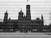 Periodic noise
 Gaussian noise
Gaussian noise is statistical noise having a probability density function (PDF) equal to that of the normal distribution, which is also known as the Gaussian distribution. In other words, the values that the noise can take on are Gaussian-distributed. The mean of this noise is approx. zero. Sometimes it is called zero-mean Gaussian noise.
Example:
Matlab
% MATLAB code for gaussian noise
% Reading the color image.
image=imread("img2.jfif");

% converting into gray.
image=rgb2gray(image);

% create the random gaussian noise of std=25
gaussian_noise=25*randn(size(image));

% display the noise
imtool(gaussian_noise,[]);

% display the gray image.
imtool(image,[]);
Output:

Example:
Matlab
% MATLAB code for demonstration of gaussian
% noisy image
% Reading the color image.
image=imread("k1.jfif");

% converting into gray.
image=rgb2gray(image);

% create the random gaussian noise of std=25
gaussian_noise=25*randn(size(image));

% display the gray image.
imtool(image,[]);

% add noise to the original image
noisy_image=double(image)+gaussian_noise;

% display the noisy image
imtool(noisy_image,[]);
Output:

Now we see how to estimate the level of Gaussian noise in the given image manually. For this firstly we generate the noisy image.
Example I:
Matlab
% MATLAB code for estimate the level of Gaussian
% noise in the given image manually
% Reading the color image.
image=imread("cameraman.jpg");

% converting into gray.
image=rgb2gray(image);

% create the random gaussian noise of std=25
gaussian_noise=25*randn(size(image));

% add noise to the original image
noisy_image=double(image)+gaussian_noise;

% display the noisy image
imtool(noisy_image,[]);
Output:

The Gaussian noise is additive in nature. That means to create the noisy image, just add the noise in the original image.
Then, we crop the homogeneous part of the image and save that. Now find the standard deviation of that part, it will give us the estimation of gaussian noise in the noisy image.
Example II:
Matlab
% MATLAB code for homogeneous part of the image
% and find the standard deviation of that part,
% it will give us the estimation of gaussian
% noise in the noisy image.
image=imread("cameraman.jpg");

% create the random gaussian noise of std=25
gaussian_noise=25*randn(size(image));

% display the gray image.
imtool(image,[]);

% add noise to the original image
noisy_image=double(image)+gaussian_noise;

% display the noisy image
imtool(noisy_image,[]);

% crop the homogeneous part of the noisy image.
% display the cropped part.
imtool(cropped_image,[]);

% standard deviation of the noise.
std(noise(:))

% standard deviation of cropped homogeneous part.
std(cropped_image(:))
Output:

Now verify the result. Match the standard deviation of the noise with the obtained result. If it is approximately equal means the homogeneous part cropped was correct otherwise choose the different homogeneous part. It requires expertise to find the perfect homogeneous part in the image.
That is why manual estimation is really time-consuming process. Next, we will see how to automate this.
How to automate the estimation of gaussian noise in the image?
We will crop the homogeneous parts from the image and calculate their standard deviations. The homogeneous part of the image will always give the same standard deviation. So, in the list of many standard deviations, the most frequently occurring will belong to the homogeneous part or we can say noise.
Thus, the idea is to take the mode of the standard deviations obtained by the sliding window. This is the automatic approach.
Step 1: Create a sliding window. Slide it over the image and find the standard deviation of them.
Step 2: Find the mode.
Note: Choose the size of the sliding window carefully. It should be chosen with respect to the size of the original noisy image. Usually, [5, 5] window is the best choice.
Example:
Matlab
% MATLAB code for automate the estimation
% of gaussian noise in the image
image=imread("cameraman.jpg");

% create the random gaussian noise of std=25
gaussian_noise=25*randn(size(image));

% add noise to the original image
noisy_image=double(image)+gaussian_noise;

% std of noise.
std(noise(:)) %output=25.1444

% list of std by using a sliding filter of [5 5].
list_of_std=uint8(colfilt(noisy_image, [5 5], 'sliding', @std));

% print the mode of this std list.
mode(list_of_std(:))
Output:
Here, the standard deviation of the noisy image is estimated as 26.
Similar Reads
Binarization of Digital Images Using Otsu Method in MATLAB
Binarization is important in digital image processing, mainly in computer vision applications. Thresholding is an efficient technique in binarization. The choice of thresholding technique is crucial in binarization. There are various thresholding algorithms have been proposed to define the optimal t
4 min read
How to add White Gaussian Noise to Signal using MATLAB ?
In this article, we are going to discuss the addition of "White Gaussian Noise" to signals like sine, cosine, and square wave using MATLAB. The white Gaussian noise can be added to the signals using MATLAB/GNU-Octave inbuilt function awgn(). Here, "AWGN" stands for "Additive White Gaussian Noise". A
4 min read
How to Remove Noise from Digital Image in Frequency Domain Using MATLAB?
Noise is defined as aberrant pixels. In other words, noise is made up of pixels not correctly representing the color or exposure of the scene. In this article, we will how to remove noise from the digital images in the frequency domain. There are two types of Noise sources Image acquisitionImage tra
5 min read
Noise addition using in-built Matlab function
Noise in an image: Digital images are prone to various types of noise that makes the quality of the images worst. Image noise is random variation of brightness or color information in the captured image. Noise is basically the degradation in image signal caused by external sources such as camera. Im
3 min read
Denoising techniques in digital image processing using MATLAB
Denoising is the process of removing or reducing the noise or artifacts from the image. Denoising makes the image more clear and enables us to see finer details in the image clearly. It does not change the brightness or contrast of the image directly, but due to the removal of artifacts, the final i
6 min read
How to Perform Random Pseudo Coloring in Grayscale Image Using MATLAB?
Pseudo Coloring is one of the attractive categories in image processing. It is used to make old black and white images or videos colorful. Pseudo Coloring techniques are used for analysis identifying color surfaces of the sample image and adaptive modeling of histogram black and white image. Selecti
3 min read
Adaptive Histogram Equalization in Image Processing Using MATLAB
Histogram Equalization is a mathematical technique to widen the dynamic range of the histogram. Sometimes the histogram is spanned over a short range, by equalization the span of the histogram is widened. In digital image processing, the contrast of an image is enhanced using this very technique. A
3 min read
How to Count the Number of Circles in Given Digital Image Using MATLAB?
In image processing, connected component analysis is the technique to count and inspect the segments automatically. Let suppose, we have an image consisting of small circles. There are hundreds of circles in the image. We need to count the number of circles. It will take a lot of time if we count ma
3 min read
Negative of an image in MATLAB
The negative of an image is achieved by replacing the intensity 'i' in the original image by 'i-1', i.e. the darkest pixels will become the brightest and the brightest pixels will become the darkest. Image negative is produced by subtracting each pixel from the maximum intensity value. For example i
2 min read
MATLAB - Image Edge Detection using Sobel Operator from Scratch
Sobel Operator: It is a discrete differentiation gradient-based operator. It computes the gradient approximation of image intensity function for image edge detection. At the pixels of an image, the Sobel operator produces either the normal to a vector or the corresponding gradient vector. It uses tw
3 min read