The probability density function(PDF) is the function that represents the density of probability for a continuous random variable over the specified ranges. It is denoted by f(x). The PDF is obtained by differentiating the Cumulative Distribution Function (CDF), and the CDF can be obtained by integrating the PDF. The PDF does not give the probability at a single point; instead, probability is found over an interval using the area under the curve.
A Probability Density Function (PDF) tells us:
- Relative Likelihood of values within a given interval
- Shape of the Distribution
- Expected Value (Mean) and Variance
A function f(x) is a valid probability density function if
- f(x) ≥ 0 for all values of x
- The total area under the curve equals 1 i.e.
\int_{-\infty}^{\infty} f(x)\,dx = 1 - The function f(x) should be piecewise continuous over its domain.
PDFs are widely used in real-life applications such as rainfall prediction, financial modeling (stock markets), and income distribution analysis.
Check:Normal distribution Formula
Example of a Probability Density Function
If the probability density function is given as:
f(x) =\begin{cases}2x, & 0 \le x \le 1 \\[5pts]0, & \text{otherwise}\end{cases}\\[5pts] Find P (0.2≤ X ≤ 0.6)
\text {Given }f(x) =\begin{cases}2x, & 0 \le x \le 1 \\[5pts]0, & \text{otherwise}\end{cases}\\[5pts]\text{Step 1: Verify that it is a valid PDF}\\[5pts]\int_{0}^{1} 2x \, dx =\left[ x^2 \right]_{0}^{1}=1\\[5pts]\text{Step 2: Find } P(0.2 \le X \le 0.6)\\[5pts] P(0.2 \le X \le 0.6)= \int_{0.2}^{0.6} 2x \, dx=\left[ x^2 \right]_{0.2}^{0.6}=[0.36 - 0.04]= 0.32\\ [5pts]\therefore \quad P(0.2 \le X \le 0.6) = 0.32
Probability Density Function Formula
Let Y be a continuous random variable and F(y) be the cumulative distribution function (CDF) of Y. Then, the probability density function (PDF) f(y) of Y is obtained by differentiating the CDF of Y.
f(y) =
\frac{d}{dy}[F(y)] = F'(y)
If we want to calculate the probability for X lying between the interval a and b, then we can use the following formula:
P (a ≤ X ≤ b) = F(b) - F(a) =
\int_{b}^{a}f(x)dx
Finding Probability Using Probability Density Function( PDF )
To find the probability from the probability density function we have to follow some steps.
Step 1: First check the PDF is valid or not using the necessary conditions.
Step 2: If the PDF is valid, use the formula and write the required probability and limits.
Step 3: Divide the integration according to the given PDF.
Step 4: Solve all integrations.
Step 5: The resultant value gives the required probability.
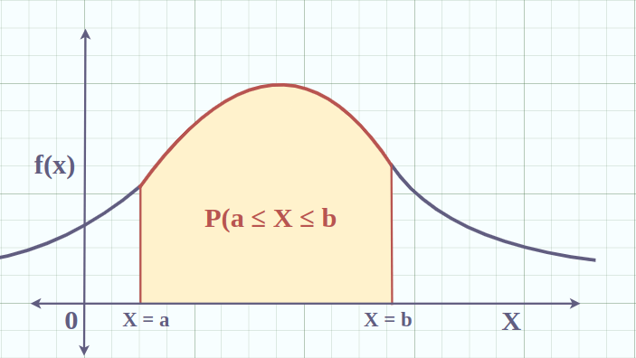
Graph for Probability Density Function
If X is continuous random variable and f(x) be the probability density function. The probability for the random variable is given by area under the PDF curve. The graph of PDF looks like bell curve, with the probability of X given by area below the curve. The following graph gives the probability for X lying between interval a and b.
Properties of Probability Density Function
Let f(x) be the probability density function for continuous random variable X.
The following are the properties of a probability density function:
- Probability density function is always positive for all the values of x : f(x) ≥ 0, ∀ x ∈ R
- Total area under probability density curve is equal to 1:
- For a continuous random variable X, probabilities are calculated over intervals. The endpoints of the interval do not affect the probability:
P (a ≤ X ≤ b) = P (a ≤ X < b) = P (a < X ≤ b) = P (a < X < b)
- Probability density function of a continuous random variable over a single value is zero.
P(X = a) = P (a ≤ X ≤ a) =
- Probability density function defines itself over the domain of the variable and over the range of the continuous values of the variable.
Important Measures of a Probability Distribution
1. Mean of Probability Density Function:
Mean of the probability density function refers to the average value of the random variable. The mean is also called as expected value or expectation. It is denoted by μ or E[X] where, X is random variable. Mean of the probability density function f(x) for the continuous random variable X is given by:
{E[X] = \mu = \int_{\infin}^{-\infin}xf(x)dx}
2. Median of Probability Density Function:
Median is the value which divides the probability density function graph into two equal halves. If x = M is the median then, area under curve from -∞ to M and area under curve from M to ∞ are equal which gives the median value = 1/2. Median of the probability density function f(x) is given by:
{\int_{M}^{-\infin}f(x)dx = \int_{\infin}^{M}f(x)dx=\frac{1}{2}}
3. Variance Probability Density Function:
Variance of probability density function refers to the squared deviation from the mean of a random variable. It is denoted by Var(X) where, X is random variable. Variance of the probability density function f(x) for continuous random variable X is given by:
Var(X) = E [(X - μ)2] =
{\int_{\infin}^{-\infin}(x-\mu)^2f(x)dx}
4. Standard Deviation of Probability Density Function
Standard Deviation is the square root of the variance. It is denoted by σ and is given by:
σ = √Var(X)
PDF Vs CDF
The key differences between Probability Density Function (PDF) and Cumulative Distribution Function (CDF) are listed in the following table:
| Probability Density Function (PDF) | Cumulative Distribution Function (CDF) |
|---|---|
| The PDF gives the probability that a random variable takes on a specific value within a certain range. | The CDF gives the probability that a random variable is less than or equal to a specific value. |
| Defined for continuous random variables. | Defined for both continuous and discrete random variables. |
| f(x), where f(x)≥0 and | F(x), where 0≤F(x)≤1 for all x, and F(−∞)=0 and F(∞)=1 |
| Represents the likelihood of the random variable taking on a specific value. | Represents cumulative probability up to a given value. |
| The area under the PDF curve over a certain interval gives the probability that the random variable falls within that interval. | The value of the CDF at a specific point gives the probability that the random variable is less than or equal to that point. |
| The PDF can be obtained by differentiating the CDF with respect to the random variable. | The CDF can be obtained by integrating the PDF with respect to the random variable. |
| The probability of a random variable falling within a specific interval (a,b) is given by | The probability of a random variable being less than or equal to a specific value x is given by |
| The PDF is always non-negative: f(x)≥0 for all x. The total area under the PDF curve is equal to 1. | The CDF is a monotonically increasing function: F(x1) ≤ F(x2) if x1 ≤ x2. 0≤F(x)≤1 for all x. |
| Normal Distribution PDF: | Normal Distribution CDF: |
Types of Probability Density Function
There are different types of probability density functions given below:
- Uniform Distribution
- Binomial Distribution
- Normal Distribution
- Chi-Square Distribution
Probability Density Function for Uniform Distribution
The uniform distribution is the distribution whose probability for equally likely events lies between a specified range. It is also called as rectangular distribution. The distribution is written as U(a, b) where, a is the minimum value and b is the maximum value. If x is the variable which lies between a and b, then formula of PDF of uniform distribution is given by:
f(x) = \frac{1}{(b - a)}
Probability Density Function for Binomial Distribution
The binomial distribution is the distribution which has two parameters: n and p where, n is the total number of trials and p is the probability of success.
Let x be the variable, n is the total number of outcomes, p is the probability of success and q be the probability of failure, then probability density function for binomial distribution is given by:
P(x) = {}^{n}C_{x} \, p^{x} q^{\,n-x}
Probability Density Function for Normal Distribution
The normal distribution is distribution that is symmetric about its mean. It is also called as Gaussian distribution. It is denoted as N (
N (
\bar{x} , σ2) = f(x) =\frac{1}{\sigma\sqrt{2\pi}}e^{\frac{-1}{2}[\frac{x - \mu}{\sigma}]^2}
In standard normal distribution mean = 0 and standard deviation = 1. So, the formula for the probability density function of the standard normal form is given by:
f(x) =
\frac{1}{\sigma\sqrt{2\pi}}e^{\frac{-x^2}{2}}
Probability Density Function for Chi-Squared Distribution
Chi-Squared distribution is the distribution defined as the sum of squares of k independent standard normal form. IT is denoted as X2(k).
The probability density function for Chi-squared distribution formula is given by:
f(x) =
\frac{x^{\frac{k}{2}-1}e^{\frac{-x}{2}}}{2^{\frac{k}{2}} \Gamma(\frac{k}{2})} , x > 0f(x) = 0, otherwise
Joint Probability Density Function
The joint probability density function is the density function that is defined for the probability distribution for two or more random variables. It is denoted as f(x, y) = Probability [(X = x) and (Y = y)] where x and y are the possible values of random variable X and Y. We can get joint PDF by differentiating joint CDF. The joint PDF must be positive and integrate to 1 over the domain.
Difference Between PDF and Joint PDF
The PDF is the function defined for single variable whereas joint PDF is the function defined for two or more than two variables, and other key differences between these both concepts are listed in the following table:
PDF (Probability Density Function) | Joint PDF |
|---|---|
Probability Density Function is the probability function defined for single variable. | Joint Probability Density Function is the probability function defined for more than one variable. |
It is denoted as f(x). | It is denoted as f (x, y, ...). |
Probability Density Function is obtained by differentiating the CDF. | Joint Probability Density Function is obtained by differentiating the joint CDF |
It can be calculated by single integral. | It can be calculated using multiple integrals as there are multiple variables. |
Read More,
Examples on Probability Density Function
Example 1: If the probability density function is given as:
Apply the formula and integrate the PDF.
P (1 ≤ X ≤ 2) =
\int_{2}^{1}f(x)dx f(x) = x / 2 for 0 ≤ x ≤ 4
⇒ P (1 ≤ X ≤ 2) =
\int_{2}^{1}(x/2)dx ⇒ P (1 ≤ X ≤ 2) =
\frac{1}{2}\times\big [\frac{x^2}{2} \big ]^2_1 ⇒ P (1 ≤ X ≤ 2) = 3 / 4
Example 2: If the probability density function is given as:
For PDF:
\int_{\infin}^{-\infin}f(x)dx = 1\\\Rightarrow\int_{1}^{-\infin}f(x)dx\hspace{0.1cm}+\hspace{0.1cm} \int_{5}^{1}f(x)dx \hspace{0.1cm}+\hspace{0.1cm} \int_{\infin}^{5}f(x)dx = 1\\\Rightarrow\int_{1}^{-\infin}0dx\hspace{0.1cm}+\hspace{0.1cm} \int_{5}^{1}c(x-1)dx \hspace{0.1cm}+\hspace{0.1cm} \int_{\infin}^{5}0dx=1\\\Rightarrow 0 \hspace{0.1cm}+\hspace{0.1cm} c \big [\frac{x^2}{2}- x\big]^5_1 +0 =1\\\Rightarrow c\big [\frac{x^2}{2}- x\big]^5_1\\\Rightarrow 8c = 1\\\Rightarrow c = \frac{1}{8}
Example 3: If the probability density function is given as:
Formula for mean:
μ =
\int_{\infin}^{-\infin}xf(x)dx ⇒ μ =
\int_{1}^{-\infin}x(0) dx\hspace{0.1cm}+\hspace{0.1cm} \int_{2}^{1} x(\frac{5x^2}{2}) dx \hspace{0.1cm}+\hspace{0.1cm} \int_{\infin}^{2}x(0) dx ⇒ μ =
\frac{5}{2}\big[\frac{x^4}{4}\big]^2_1 ⇒ μ = (5/2) × (15/4)
⇒ μ = 75/8 = 9.375
Example 4: If the probability density function is given as:
To verify that f(x) is a valid PDF, it must satisfy two conditions:
f(x)≥0 for all x.
The integral of f(x) over its entire range must equal 1.
Checking f(x)≥0:
f(x)=2x is clearly non-negative for 0≤x≤10.
Integrating f(x) over its range:∫−∞∞f(x) dx=∫012x dx=[x2]01=12−02=1.
\int_{-\infty}^{\infty} f(x) \, dx = \int_{0}^{1} 2x \, dx = \left[ x^2 \right]_{0}^{1} = 12 - 02 = 1.
Since both conditions are satisfied, f(x) is a valid PDF.
Example 5: Given the probability density function f(x)=
The mean of a continuous random variable X with PDF f(x) is given by:
E(X)=
\int_{-\infty}^{\infty} x f(x) \, dx .For the given PDF:
E(X)= =
\int_{0}^{1} x \cdot 3x^2 \, dx =
\int_{0}^{1} 3x^3 \, dx =
3 \left[ \frac{x^4}{4} \right]_{0}^{1} =
3 \cdot \frac{1}{4} =
\frac{3}{4}
Example 6: Using the same PDF
The variance of a continuous random variable X is given by:
\text{Var}(X) = E(X^2) - [E(X)]^2. We already have
E(X) = \frac{3}{4} .Now, we need to find E(X2):
E(X^2) = \int_{-\infty}^{\infty} x^2 f(x) \, dx
= \int_{0}^{1} x^2 \cdot 3x^2 \, dx
= \int_{0}^{1} 3x^4 \, dx
= 3 \left[ \frac{x^5}{5} \right]_{0}^{1}
= 3 \cdot \frac{1}{5}
= \frac{3}{5}.
Practice Questions on Probability Density Function
Q 1: Let f(x) be a probability density function given by:
- f(x) = 2x for 0 ≤ x ≤ 2
- f(x) = 0 otherwise
Verify that f(x) is a valid probability density function.
Q 2: Let f(x) be a probability density function given by:
- f(x) = 1/2e-x/2 for x ≥ 0
- f(x) = 0 for x < 0
Calculate the probability that X ≤ 1.
Q 3: Let f(x) be a probability density function given by:
- f(x) = 2x2 for 0 ≤ x ≤ 1
- f(x) = 0 otherwise
Find the cumulative distribution function (CDF) F(x) for x ≥ 0.
Q 4: Given the function
Q 5: For the PDF