�Ettore Majorana: Unpublished Research Notes on Theoretical Physics
�Fundamental Theories of Physics
An International Book Series on The Fundamental Theories of Physics:
Their Clarification, Development and Application
Series Editors:
GIANCARLO GHIRARDI, University of Trieste, Italy
VESSELIN PETKOV, Concordia University, Canada
TONY SUDBERY, University of York, UK
ALWYN VAN DER MERWE, University of Denver, CO, USA
Volume 159
For other titles published in this series, go to www.springer.com/series/6001
�Ettore Majorana:
Unpublished Research Notes
on Theoretical Physics
Edited by
S. Esposito
University of Naples “Federico II”
Italy
E. Recami
University of Bergamo
Italy
A. van der Merwe
University of Denver
Colorado, USA
R. Battiston
University of Perugia
Italy
�Editors
Salvatore Esposito Alwyn van der Merwe
Università di Napoli “Federico II” University of Denver
Dipartimento di Scienze Fisiche Department of Physics and Astronomy
Complesso Universitario di Monte S. Angelo Denver, CO 80208
Via Cinthia USA
80126 Napoli
Italy
Erasmo Recami Roberto Battiston
Università di Bergamo Università di Perugia
Facoltà di Ingegneria Dipartimento di Fisica
24044 Dalmine (BG) Via A. Pascoli
Italy 06123 Perugia
Italy
Back cover photo of E. Majorana: Copyright by E. Recami & M. Majorana, reproduction of the photo is
not allowed (without written permission of the right holders)
ISBN 978-1-4020-9113-1 e-ISBN 978-1-4020-9114-8
Library of Congress Control Number: 2008935622
�c 2009 Springer Science + Business Media B.V.
No part of this work may be reproduced, stored in a retrieval system, or transmitted in any form or by any
means, electronic, mechanical, photocopying, microfilming, recording or otherwise, without the written
permission from the Publisher, with the exception of any material supplied specifically for the purpose of
being entered and executed on a computer system, for the exclusive use by the purchaser of the work.
Printed on acid-free paper
9 8 7 6 5 4 3 2 1
springer.com
�“But, then, there are geniuses like Galileo and Newton.
Well, Ettore Majorana was one of them...”
Enrico Fermi (1938)
�CONTENTS
Preface xiii
Bibliography xxxvii
Table of contents of the complete set of Majorana’s Quaderni
(ca. 1927-1933) xliii
CONTENTS OF THE SELECTED MATERIAL
Part I
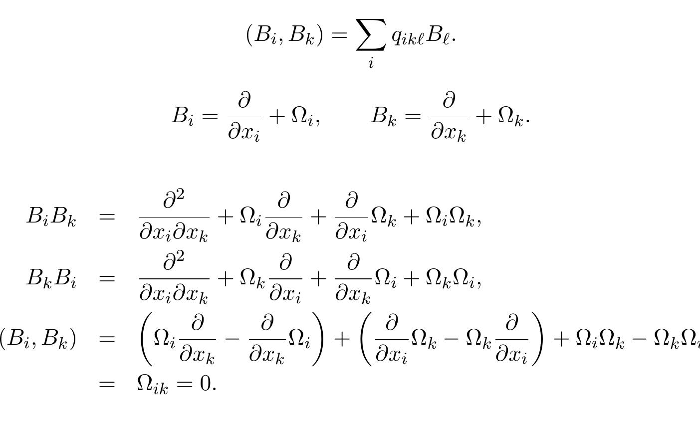
Dirac Theory 3
1.1 Vibrating string [Q02p038] 3
1.2 A semiclassical theory for the electron [Q02p039] 4
1.2.1 Relativistic dynamics 4
1.2.2 Field equations 7
1.3 Quantization of the Dirac field [Q01p133] 22
1.4 Interacting Dirac fields [Q02p137] 25
1.4.1 Dirac equation 25
1.4.2 Maxwell equations 27
1.4.3 Maxwell-Dirac theory 29
1.4.3.1 Normal mode decomposition 31
1.4.3.2 Particular representations of Dirac operators 32
1.5 Symmetrization [Q02p146] 35
1.6 Preliminaries for a Dirac equation in real terms [Q13p003] 35
1.6.1 First formalism 36
1.6.2 Second formalism 38
1.6.3 Angular momentum 40
1.6.4 Plane-wave expansion 44
1.6.5 Real fields 45
1.6.6 Interaction with an electromagnetic field 45
vii
�viii E. MAJORANA: RESEARCH NOTES ON THEORETICAL PHYSICS
1.7 Dirac-like equations for particles with spin higher than 1/2
[Q04p154] 47
1.7.1 Spin-1/2 particles (4-component spinors) 47
1.7.2 Spin-7/2 particles (16-component spinors) 48
1.7.3 Spin-1 particles (6-component spinors) 48
1.7.4 5-component spinors 55
Quantum Electrodynamics 57
2.1 Basic lagrangian and hamiltonian formalism for the electro-
magnetic field [Q01p066] 57
2.2 Analogy between the electromagnetic field and the Dirac field
[Q02a101] 59
2.3 Electromagnetic field: plane wave operators [Q01p068] 64
2.3.1 Dirac formalism 68
2.4 Quantization of the electromagnetic field [Q03p061] 71
2.5 Continuation I: angular momentum [Q03p155] 78
2.6 Continuation II: including the matter fields [Q03p067] 82
2.7 Quantum dynamics of electrons interacting with an electro-
magnetic field [Q02p102] 84
2.8 Continuation [Q02p037] 94
2.9 Quantized radiation field [Q17p129b] 95
2.10 Wave equation of light quanta [Q17p142] 100
2.11 Continuation [Q17p151] 101
2.12 Free electron scattering [Q17p133] 104
2.13 Bound electron scattering [Q17p142] 112
2.14 Retarded fields [Q05p065] 116
2.14.1 Time delay 118
2.15 Magnetic charges [Q03p163] 119
Appendix: Potential experienced by an electric charge [Q02p101] 121
Part II
Atomic Physics 125
3.1 Ground state energy of a two-electron atom [Q12p058] 125
3.1.1 Perturbation method 125
3.1.2 Variational method 128
3.1.2.1 First case 129
3.1.2.2 Second case 130
3.1.2.3 Third case 131
3.2 Wavefunctions of a two-electron atom [Q17p152] 133
3.3 Continuation: wavefunctions for the helium atom [Q05p156] 136
3.4 Self-consistent field in two-electron atoms [Q16p100] 141
3.5 2s terms for two-electron atoms [Q16p157b] 144
3.6 Energy levels for two-electron atoms [Q07p004] 144
3.6.1 Preliminaries for the X and Y terms 148
�CONTENTS ix
3.6.2 Simple terms 151
3.6.3 Electrostatic energy of the 2s2p term 155
3.6.4 Perturbation theory for s terms 157
3.6.5 2s2p 3 P term 158
3.6.6 X term 159
3.6.7 2s2s 1 S and 2p2p 1 S terms 169
3.6.8 1s1s term 170
3.6.9 1s2s term 174
3.6.10 Continuation 175
3.6.11 Other terms 176
3.7 Ground state of three-electron atoms [Q16p157a] 183
3.8 Ground state of the lithium atom [Q16p098] 184
3.8.1 Electrostatic potential 184
3.8.2 Ground state 185
3.9 Asymptotic behavior for the s terms in alkali [Q16p158] 190
3.9.1 First method 191
3.9.2 Second method 195
3.10 Atomic eigenfunctions I [Q02p130] 197
3.11 Atomic eigenfunctions II [Q17p161] 201
3.12 Atomic energy tables [Q06p026] 204
3.13 Polarization forces in alkalies [Q16p049] 205
3.14 Complex spectra and hyperfine structures [Q05p051] 211
3.15 Calculations about complex spectra [Q05p131] 219
3.16 Resonance between a p (ℓ = 1) electron and an electron with
azimuthal quantum number ℓ′ [Q07p117] 223
3.16.1 Resonance between a d electron and a p shell I 224
3.16.2 Eigenfunctions of d 5 , d 3 , p 3 and p 1 electrons 225
2 2 2 2
3.16.3 Resonance between a d electron and a p shell II 227
3.17 Magnetic moment and diamagnetic susceptibility for a one-
electron atom (relativistic calculation) [Q17p036] 229
3.18 Theory of incomplete P ′ triplets [Q07p061] 233
3.18.1 Spin-orbit couplings and energy levels 233
3.18.2 Spectral lines for Mg and Zn 237
3.18.3 Spectral lines for Zn, Cd and Hg 238
3.19 Hyperfine structure: relativistic Rydberg corrections [Q04p143] 239
3.20 Non-relativistic approximation of Dirac equation for a two-
particle system [Q04p149] 242
3.20.1 Non-relativistic decomposition 243
3.20.2 Electromagnetic interaction between two charged par-
ticles 244
3.20.3 Radial equations 245
3.21 Hyperfine structures and magnetic moments: formulae and ta-
bles [Q04p165] 246
3.22 Hyperfine structures and magnetic moments: calculations
[Q04p169] 251
3.22.1 First method 251
3.22.2 Second method 254
�x E. MAJORANA: RESEARCH NOTES ON THEORETICAL PHYSICS
Molecular Physics 261
4.1 The helium molecule [Q16p001] 261
4.1.1 The equation for σ -electrons in elliptic coordinates 261
4.1.2 Evaluation of P2 for s-electrons: relation between W
and λ 263
4.1.3 Evaluation of P1 275
4.2 Vibration modes in molecules [Q06p031] 275
4.2.1 The acetylene molecule 278
4.3 Reduction of a three-fermion to a two-particle system [Q03p176] 282
Statistical Mechanics 287
5.1 Degenerate gas [Q17p097] 287
5.2 Pauli paramagnetism [Q18p157] 288
5.3 Ferromagnetism [Q08p014] 289
5.4 Ferromagnetism: applications [Q08p046] 300
5.5 Again on ferromagnetism [Q06p008] 307
Part III
The Theory of Scattering 311
6.1 Scattering from a potential well [Q06p015] 311
6.2 Simple perturbation method [Q06p024] 316
6.3 The Dirac method [Q01p106] 317
6.3.1 Coulomb field 318
6.4 The Born method [Q01p109] 319
6.5 Coulomb scattering [Q01p010] 321
6.6 Quasi coulombian scattering of particles [Q01p001] 324
6.6.1 Method of the particular solutions 327
6.7 Coulomb scattering: another regularization method [Q01p008] 328
6.8 Two-electron scattering [Q03p029] 330
6.9 Compton effect [Q03p041] 331
6.10 Quasi-stationary states [Q03p103] 332
Appendix: Transforming a differential equation [Q03p035] 337
Nuclear Physics 339
7.1 Wave equation for the neutron [Q17p129] 339
7.2 Radioactivity [Q17p005] 339
7.3 Nuclear potential [Q17p006] 340
7.3.1 Mean nucleon potential 340
7.3.2 Computation of the interaction potential between nu-
cleons 342
7.3.3 Nucleon density 345
�CONTENTS xi
7.3.4 Nucleon interaction I 347
7.3.4.1 Zeroth approximation 351
7.3.5 Nucleon interaction II 352
7.3.5.1 Evaluation of some integrals 355
7.3.5.2 Zeroth approximation 358
7.3.6 Simple nuclei I 363
7.3.7 Simple nuclei II 365
7.3.7.1 Kinematics of two α particles (statistics) 367
7.4 Thomson formula for β particles in a medium [Q16p083] 368
7.5 Systems with two fermions and one boson [Q17p090] 370
7.6 Scalar field theory for nuclei? [Q02p086] 370
Part IV
Classical Physics 385
8.1 Surface waves in a liquid [Q12p054] 385
8.2 Thomson’s method for the determination of e/m [Q09p044[ 387
8.3 Wien’s method for the determination of e/m (positive charges)
[Q09p048b] 388
8.4 Determination of the electron charge [Q09p028] 390
8.4.1 Townsend effect 390
8.4.1.1 Ion recombination 390
8.4.1.2 Ion diffusion 392
8.4.1.3 Velocity in the electric field 393
8.4.1.4 Charge of an ion 393
8.4.2 Method of the electrolysis (Townsend) 394
8.4.3 Zaliny’s method for the ratio of the mobility coefficients 394
8.4.4 Thomson’s method 395
8.4.5 Wilson’s method 396
8.4.6 Millikan’s method 396
8.5 Electromagnetic and electrostatic mass of the electron
[Q09p048] 397
8.6 Thermionic effect [Q09p053] 397
8.6.1 Langmuir Experiment on the effect of the electron cloud 399
Mathematical Physics 403
9.1 Linear partial differential equations. Complete systems
[Q11p087] 403
9.1.1 Linear operators 404
9.1.2 Integrals of an ordinary differential system and the par-
tial differential equation which determines them 405
9.1.3 Integrals of a total differential system and the associ-
ated system of partial differential equation that deter-
mines them 406
9.2 Algebraic foundations of the tensor calculus [Q11p093] 409
9.2.1 Covariant and contravariant vectors 409
�xii E. MAJORANA: RESEARCH NOTES ON THEORETICAL PHYSICS
9.3 Geometrical introduction to the theory of differential quadratic
forms I [Q11p094] 409
9.3.1 The symbolic equation of parallelism 409
9.3.2 Intrinsic equations of parallelism 409
9.3.3 Christoffel’s symbols 411
9.3.4 Equations of parallelism in terms of covariant compo-
nents 412
9.3.5 Some analytical verifications 413
9.3.6 Permutability 414
9.3.7 Line elements 414
9.3.8 Euclidean manifolds. any Vn can always be considered
as immersed in a Euclidean space 415
9.3.9 Angular metric 416
9.3.10 Coordinate lines 417
9.3.11 Differential equations of geodesics 418
9.3.12 Application 420
9.4 Geometrical introduction to the theory of differential quadratic
forms II [Q11p113] 422
9.4.1 Geodesic curvature 422
9.4.2 Vector displacement 422
9.4.3 Autoparallelism of geodesics 424
9.4.4 Associated vectors 424
9.4.5 Remarks on the case of an indefinite ds2 425
9.5 Covariant differentiation. Invariants and differential parame-
ters. Locally geodesic coordinates [Q11p119] 425
9.5.1 Geodesic coordinates 425
9.5.1.1 Applications 427
9.5.2 Particular cases 429
9.5.3 Applications 430
9.5.4 Divergence of a vector 431
9.5.5 Divergence of a double (contravariant) tensor 432
9.5.6 Some laws of transformation 433
9.5.7 ε systems 434
9.5.8 Vector product 435
9.5.9 Extension of a field 435
9.5.10 Curl of a vector in three dimensions 436
9.5.11 Sections of a manifold. Geodesic manifolds 436
9.5.12 Geodesic coordinates along a given line 437
9.6 Riemann’s symbols and properties relating to curvature
[Q11p138] 441
9.6.1 Cyclic displacement round an elementary parallelogram 441
9.6.2 Fundamental properties of Riemann’s symbols of the
second kind 443
9.6.3 Fundamental properties and number of Riemann’s sym-
bols of the first kind 444
9.6.4 Bianchi identity and Ricci lemma 447
9.6.5 Tangent geodesic coordinates around the point P0 447
Index 449
�Preface
Without listing his works, all of which are highly notable both for the
originality of the methods utilized as well as for the importance of the
results achieved, we limit ourselves to the following:
In modern nuclear theories, the contribution made by this researcher
to the introduction of the forces called ‘Majorana forces’ is universally
recognized as the one, among the most fundamental, that permits us
to theoretically comprehend the reasons for nuclear stability. The work
of Majorana today serves as a basis for the most important research in
this field.
In atomic physics, the merit of having resolved some of the most in-
tricate questions on the structure of spectra through simple and elegant
considerations of symmetry is due to Majorana.
Lastly, he devised a brilliant method that permits us to treat the
positive and negative electron in a symmetrical way, finally eliminat-
ing the necessity to rely on the extremely artificial and unsatisfactory
hypothesis of an infinitely large electrical charge diffused in space, a
question that had been tackled in vain by many other scholars [4].
With this justification, the judging committee of the 1937 competition
for a new full professorship in theoretical physics at Palermo, chaired
by Enrico Fermi (and including Enrico Persico, Giovanni Polvani and
Antonio Carrelli), suggested the Italian Minister of National Educa-
tion should appoint Ettore Majorana “independently of the competition
rules, as full professor of theoretical physics in a university of the Italian
kingdom1 because of his high and well-deserved reputation” [4]. Evi-
dently, to gain such a high reputation the few papers that the Italian
scientist had chosen to publish were enough. It is interesting to note that
proper light was shed by Fermi on Majorana’s symmetrical approach to
electrons and antielectrons (today climaxing in its application to neu-
trinos and antineutrinos) and on its ability to eliminate the hypothesis
1 Which happened to be the University of Naples.
xiii
�xiv E. MAJORANA: RESEARCH NOTES ON THEORETICAL PHYSICS
known as the “Dirac sea”, a hypothesis that Fermi defined as “extremely
artificial and unsatisfactory”, despite the fact that in general it had been
uncritically accepted. However, one of the most important works of Ma-
jorana, the one that introduced his “infinite-components equation” was
not mentioned: it had not been understood yet, even by Fermi and his
colleagues.
Bruno Pontecorvo [2], a younger colleague of Majorana at the Institute
of Physics in Rome, in a similar way recalled that “some time after his
entry into Fermi’s group, Majorana already possessed such an erudition
and had reached such a high level of comprehension of physics that he
was able to speak on the same level with Fermi about scientific problems.
Fermi himself held him to be the greatest theoretical physicist of our
time. He often was astounded ....”
Majorana’s fame rests solidly on testimonies like these, and even more
on the following ones.
At the request of Edoardo Amaldi [1], Giuseppe Cocconi wrote from
CERN (18 July 1965):
In January 1938, after having just graduated, I was invited, essentially
by you, to come to the Institute of Physics at the University of Rome
for six months as a teaching assistant, and once I was there I would have
the good fortune of joining Fermi, Gilberto Bernardini (who had been
given a chair at Camerino University a few months earlier) and Mario
Ageno (he, too, a new graduate) in the research of the products of
disintegration of μ “mesons” (at that time called mesotrons or yukons),
which are produced by cosmic rays....
A few months later, while I was still with Fermi in our workshop,
news arrived of Ettore Majorana’s disappearance in Naples. I remember
that Fermi busied himself with telephoning around until, after some
days, he had the impression that Ettore would never be found.
It was then that Fermi, trying to make me understand the sig-
nificance of this loss, expressed himself in quite a peculiar way; he who
was so objectively harsh when judging people. And so, at this point, I
would like to repeat his words, just as I can still hear them ringing in my
memory: ‘Because, you see, in the world there are various categories of
scientists: people of a secondary or tertiary standing, who do their best
but do not go very far. There are also those of high standing, who come
to discoveries of great importance, fundamental for the development of
science’ (and here I had the impression that he placed himself in that
category). ‘But then there are geniuses like Galileo and Newton. Well,
Ettore was one of them. Majorana had what no one else in the world
had ...’.
Fermi, who was rather severe in his judgements, again expressed him-
self in an unusual way on another occasion. On 27 July 1938 (after
�PREFACE xv
Majorana’s disappearance, which took place on 26 March 1938), writing
from Rome to Prime Minister Mussolini to ask for an intensification of
the search for Majorana, he stated: “I do not hesitate to declare, and it
would not be an overstatement in doing so, that of all the Italian and
foreign scholars that I have had the chance to meet, Majorana, for his
depth of intellect, has struck me the most” [4].
But, nowadays, some interested scholars may find it difficult to ap-
preciate Majorana’s ingeniousness when basing their judgement only on
his few published papers (listed below), most of them originally written
in Italian and not easy to trace, with only three of his articles having
been translated into English [9, 10, 11, 12, 28] in the past. Actually,
only in 2006 did the Italian Physical Society eventually publish a book
with the Italian and English versions of Majorana’s articles [13].
Anyway, Majorana has also left a lot of unpublished manuscripts
relating to his studies and research, mainly deposited at the Domus
Galilaeana in Pisa (Italy), which help to illuminate his abilities as a
theoretical physicist, and mathematician too.
The year 2006 was the 100th anniversary of the birth of Ettore
Majorana, probably the brightest Italian theoretician of the twentieth
century, even though to many people Majorana is known mainly for his
mysterious disappearance, in 1938, at the age of 31. To celebrate such
a centenary, we had been working—among others—on selection, study,
typographical setting in electronic form and translation into English of
the most important research notes left unpublished by Majorana: his
so-called Quaderni (booklets); leaving aside, for the moment, the no-
table set of loose sheets that constitute a conspicuous part of Majo-
rana’s manuscripts. Such a selection is published for the first time,
with some understandable delay, in this book. In a previous volume
[15], entitled Ettore Majorana: Notes on Theoretical Physics, we anal-
ogously published for the first time the material contained in different
Majorana booklets—the so-called Volumetti, which had been written by
him mainly while studying physics and mathematics as a student and
collaborator of Fermi. Even though Ettore Majorana: Notes on Theo-
retical Physics contained many highly original findings, the preparation
of the present book remained nevertheless a rather necessary enterprise,
since the research notes publicited in it are even more (and often ex-
ceptionally) interesting, revealing more fully Majorana’s genius. Many
of the results we will cover on the hundreds of pages that follow are
novel and even today, more than seven decades later, still of significant
importance for contemporary theoretical physics.
�xvi E. MAJORANA: RESEARCH NOTES ON THEORETICAL PHYSICS
Historical prelude
For nonspecialists, the name of Ettore Majorana is frequently associated
with his mysterious disappearance from Naples, on 26 March 1938, when
he was only 31; afterwards, in fact, he was never seen again.
But the myth of his “disappearance” [4] has contributed to nothing
but the fame he was entitled to, for being a genius well ahead of his time.
Ettore Majorana was born on 5 August 1906 at Catania, Sicily
(Italy), to Fabio Majorana and Dorina Corso. The fourth of five sons,
he had a rich scientific, technological and political heritage: three of
his uncles had become vice-chancellors of the University of Catania and
members of the Italian parliament, while another, Quirino Majorana,
was a renowned experimental physicist, who had been, by the way, a
former president of the Italian Physical Society.
Ettore’s father, Fabio, was an engineer who had founded the first
telephone company in Sicily and who went on to become chief inspector
of the Ministry of Communications. Fabio Majorana was responsible for
the education of his son in the first years of his school-life, but afterwards
Ettore was sent to study at a boarding school in Rome. Eventually, in
1921, the whole family moved from Catania to Rome. Ettore finished
high school in 1923 when he was 17, and then joined the Faculty of
Engineering of the local university, where he excelled, and counted Gio-
vanni Gentile Jr., Enrico Volterra, Giovanni Enriques and future Nobel
laureate Emilio Segr`e among his friends.
In the spring of 1927 Orso Mario Corbino, the director of the In-
stitute of Physics at Rome and an influential politician (who had suc-
ceeded in elevating to full professorship the 25-year-old Enrico Fermi,
just with the intention of enabling Italian physics to make a quality
jump) launched an appeal to the students of the Faculty of Engineer-
ing, inviting the most brilliant young minds to study physics. Segr`e
and Edoardo Amaldi rose to the challenge, joining Fermi and Franco
Rasetti’s group, and telling them of Majorana’s exceptional gifts. Af-
ter some encouragement from Segr`e and Amaldi, Majorana eventually
decided to meet Fermi in the autumn of that year.
The details of Majorana and Fermi’s first meeting were narrated
by Segr´e [3], Rasetti and Amaldi. The first important work written
by Fermi in Rome, on the statistical properties of the atom, is today
known as the Thomas–Fermi method. Fermi had found that he needed
the solution to a nonlinear differential equation characterized by unusual
boundary conditions, and in a week of assiduous work he had calculated
the solution with a little hand calculator. When Majorana met Fermi
for the first time, the latter spoke about his equation, and showed his
�PREFACE xvii
numerical results. Majorana, who was always very sceptical, believed
Fermi’s numerical solution was probably wrong. He went home, and
solved Fermi’s original equation in analytic form, evaluating afterwards
the solution’s values without the aid of a calculator. Next morning he
returned to the Institute and sceptically compared the results which he
had written on a little piece of paper with those in Fermi’s notebook,
and found that their results coincided exactly. He could not hide his
amazement, and decided to move from the Faculty of Engineering to
the Faculty of Physics. We have indulged ourselves in the foregoing
anecdote since the pages on which Majorana solved Fermi’s differential
equation were found by one of us (S.E.) years ago. And recently [22]
it was explicitly shown that he followed that night two independent
paths, the first of them leading to an Abel equation, and the second one
resulting in his devising a method still unknown to mathematics. More
precisely, Majorana arrived at a series solution of the Thomas–Fermi
equation by using an original method that applies to an entire class of
mathematical problems. While some of Majorana’s results anticipated
by several years those of renowned mathematicians or physicists, several
others (including his final solution to the equation mentioned) have not
been obtained by anyone else since. Such facts are further evidence of
Majorana’s brilliance.
Majorana’s published articles
Majorana published few scientific articles: nine, actually, besides his so-
ciology paper entitled “Il valore delle leggi statistiche nella fisica e nelle
scienze sociali” (“The value of statistical laws in physics and the social
sciences”), which was, however, published not by Majorana but (posthu-
mously) by G. Gentile Jr., in Scientia (36:55–56, 1942), and much later
was translated into English. Majorana switched from engineering to
physics studies in 1928 (the year in which he published his first article,
written in collaboration with his friend Gentile) and then went on to
publish his works on theoretical physics for only a few years, practically
only until 1933. Nevertheless, even his published works are a mine of
ideas and techniques of theoretical physics that still remain largely un-
explored. Let us list his nine published articles, which only in 2006 were
eventually reprinted together with their English translations [13]:
1. Sullo sdoppiamento dei termini Roentgen ottici a causa dell’elet-
trone rotante e sulla intensit`
a delle righe del Cesio, Rendiconti Ac-
cademia Lincei 8, 229–233 (1928) (in collaboration with Giovanni
Gentile Jr.)
�xviii E. MAJORANA: RESEARCH NOTES ON THEORETICAL PHYSICS
2. Sulla formazione dello ione molecolare di He, Nuovo Cimento 8,
22–28 (1931)
3. I presunti termini anomali dell’Elio, Nuovo Cimento 8, 78–83 (1931)
4. Reazione pseudopolare fra atomi di Idrogeno, Rendiconti Accademia
Lincei 13, 58–61 (1931)
5. Teoria dei tripletti P’ incompleti, Nuovo Cimento 8, 107–113 (1931)
6. Atomi orientati in campo magnetico variabile, Nuovo Cimento 9,
43–50 (1932)
7. Teoria relativistica di particelle con momento intrinseco arbitrario,
Nuovo Cimento 9, 335–344 (1932)
¨
8. Uber die Kerntheorie, Zeitschrift f¨ur Physik 82, 137–145 (1933);
Sulla teoria dei nuclei, La Ricerca Scientifica 4(1), 559–565 (1933)
9. Teoria simmetrica dell’elettrone e del positrone, Nuovo Cimento
14, 171–184 (1937)
While still an undergraduate, in 1928 Majorana published his first
paper, (1), in which he calculated the splitting of certain spectroscopic
terms in gadolinium, uranium and caesium, owing to the spin of the
electrons. At the end of that same year, Fermi invited Majorana to
give a talk at the Italian Physical Society on some applications of the
Thomas–Fermi model [23] (attention to which was drawn by F. Guerra
and N. Robotti). Then on 6 July 1929, Majorana was awarded his
master’s degree in physics, with a dissertation having as a subject “The
quantum theory of radioactive nuclei”.
By the end of 1931 the 25-year-old physicist had published two ar-
ticles, (2) and (4), on the chemical bonds of molecules, and two more pa-
pers, (3) and (5), on spectroscopy, one of which, (3), anticipated results
later obtained by a collaborator of Samuel Goudsmith on the “Auger
effect” in helium. As Amaldi has written, an in-depth examination of
these works leaves one struck by their quality: they reveal both deep
knowledge of the experimental data, even in the minutest detail, and an
uncommon ease, without equal at that time, in the use of the symmetry
properties of the quantum states to qualitatively simplify problems and
choose the most suitable method for their quantitative resolution.
In 1932, Majorana published an important paper, (6), on the nona-
diabatic spin-flip of atoms in a magnetic field, which was later extended
by Nobel laureate Rabi in 1937, and by Bloch and Rabi in 1945. It
established the theoretical basis for the experimental method used to re-
verse the spin also of neutrons by a radio-frequency field, a method that
�PREFACE xix
is still practised today, for example, in all polarized-neutron spectrome-
ters. That paper contained an independent derivation of the well-known
Landau–Zener formula (1932) for nonadiabatic transition probability.
It also introduced a novel mathematical tool for representing spherical
functions or, rather, for representing spinors by a set of points on the
surface of a sphere (Majorana sphere), attention to which was drawn not
long ago by Penrose and collaborators [29] (and by Leonardi and cowork-
ers [30]). In the present volume the reader will find some additions (or
modifications) to the above-mentioned published articles.
However, the most important 1932 paper is that concerning a rela-
tivistic field theory of particles with arbitrary spin, (7). Around 1932 it
was commonly believed that one could write relativistic quantum equa-
tions only in the case of particles with spin 0 or 1/2. Convinced of
the contrary, Majorana—as we have known for a long time from his
manuscripts, constituting a part of the Quaderni finally published here—
began constructing suitable quantum-relativistic equations for higher
spin values (1, 3/2, etc.); and he even devised a method for writing
the equation for a generic spin value. But still he published nothing,2
until he discovered that one could write a single equation to cover an
infinite family of particles of arbitrary spin (even though at that time
the known particles could be counted on one hand). To implement his
programme with these “infinite-components” equations, Majorana in-
vented a technique for the representation of a group several years before
Eugene Wigner did. And, what is more, Majorana obtained the infinite-
dimensional unitary representations of the Lorentz group that would be
rediscovered by Wigner in his 1939 and 1948 works. The entire the-
ory was reinvented in a Soviet series of articles from 1948 to 1958, and
finally applied by physicists years later. Sadly, Majorana’s initial ar-
ticle remained in the shadows for a good 34 years until Fradkin [28],
informed by Amaldi, realized what Majorana many years earlier had
accomplished. All the scientific material contained in (and in prepa-
ration for) this publication of Majorana’s works is illuminated by the
manuscripts published in the present volume.
At the beginning of 1932, as soon as the news of the Joliot–Curie
experiments reached Rome, Majorana understood that they had discov-
ered the “neutral proton” without having realized it. Thus, even before
the official announcement of the discovery of the neutron, made soon af-
terwards by Chadwick, Majorana was able to explain the structure and
stability of light atomic nuclei with the help of protons and neutrons,
2 Starting
in 1974, some of us [21] published and revaluated only a few of the pages devoted
in Majorana’s manuscripts to the case of a Dirac-like equation for the photon (spin-1 case).
�xx E. MAJORANA: RESEARCH NOTES ON THEORETICAL PHYSICS
antedating in this way also the pioneering work of D. Ivanenko, as both
Segr´e and Amaldi have recounted. Majorana’s colleagues remember that
even before Easter he had concluded that protons and neutrons (indis-
tinguishable with respect to the nuclear interaction) were bound by the
“exchange forces” originating from the exchange of their spatial positions
alone (and not also of their spins, as Heisenberg would propose), so as to
produce the α particle (and not the deuteron) as saturated with respect
to the binding energy. Only after Heisenberg had published his own arti-
cle on the same problem was Fermi able to persuade Majorana to go for a
6-month period, in 1933, to Leipzig and meet there his famous colleague
(who would be awarded the Nobel prize at the end of that year); and fi-
nally Heisenberg was able to convince Majorana to publish his results in
¨
the paper “Uber die Kerntheorie”. Actually, Heisenberg had interpreted
the nuclear forces in terms of nucleons exchanging spinless electrons, as if
the neutron were formed in practice by a proton and an electron, whereas
Majorana had simply considered the neutron as a “neutral proton”, and
the theoretical and experimental consequences were quickly recognized
by Heisenberg. Majorana’s paper on the stability of nuclei soon became
known to the scientific community—a rare event, as we know—thanks to
that timely “propaganda” made by Heisenberg himself, who on several
occasions, when discussing the “Heisenberg–Majorana” exchange forces,
used, rather fairly and generously, to point out more Majorana’s than his
own contributions [33]. The manuscripts published in the present book
refer also to what Majorana wrote down before having read Heisenberg’s
paper. Let us seize the present opportunity to quote two brief passages
from Majorana’s letters from Leipzig. On 14 February 1933, he wrote
to his mother (the italics are ours): “The environment of the physics
institute is very nice. I have good relations with Heisenberg, with Hund,
and with everyone else. I am writing some articles in German. The
first one is already ready ...” [4]. The work that was already ready is,
naturally, the cited one on nuclear forces, which, however, remained the
only paper in German. Again, in a letter dated 18 February, he told his
father (our italics): “I will publish in German, after having extended it,
also my latest article which appeared in Il Nuovo Cimento” [4].
But Majorana published nothing more, either in Germany—where
he had become acquainted, besides with Heisenberg, with other renowned
scientists, including Ehrenfest, Bohr, Weisskopf and Bloch—or after his
return to Italy, except for the article (in 1937) of which we are about to
speak. It is therefore important to know that Majorana was engaged in
writing other papers: in particular, he was expanding his article about
the infinite-components equations. His research activity during the years
1933–1937 is testified by the documents presented in this volume, and
�PREFACE xxi
particularly by a number of unpublished scientific notes, some of which
are reproduced here: as far as we know, it focused mainly on field theory
and quantum electrodynamics. As already mentioned, in 1937 Majorana
decided to compete for a full professorship (probably with the only de-
sire to have students); and he was urged to demonstrate that he was still
actively working in theoretical physics. Happily enough, he took from a
drawer3 his writing on the symmetrical theory of electrons and antielec-
trons, publishing it that same year under the title “Symmetric theory
of electrons and positrons”. This paper—at present probably the most
famous of his—was initially noticed almost exclusively for having intro-
duced the Majorana representation of the Dirac matrices in real form.
But its main consequence is that a neutral fermion can be identical with
its antiparticle. Let us stress that such a theory was rather revolution-
ary, since it was at variance with what Dirac had successfully assumed
in order to solve the problem of negative energy states in quantum field
theory. With rare daring, Majorana suggested that neutrinos, which had
just been postulated by Pauli and Fermi to explain puzzling features of
radioactive β decay, could be particles of this type. This would enable
the neutrino, for instance, to have mass, which may have a bearing on
the phenomena of neutrino oscillations, later postulated by Pontecorvo.
It may be stressed that, exactly as in the case of other writings
of his, the “Majorana neutrino” too started to gain prominence only
decades later, beginning in the 1950s; and nowadays expressions such
as Majorana spinors, Majorana mass and even “majorons” are fashion-
able. It is moreover well known that many experiments are currently
devoted the world over to checking whether the neutrinos are of the
Dirac or the Majorana type. We have already said that the material
published by Majorana (but still little known, despite everything) con-
stitutes a potential gold mine for physics. Many years ago, for exam-
ple, Bruno Touschek noticed that the article entitled “Symmetric theory
of electrons and positrons” implicitly contains also what he called the
theory of the “Majorana oscillator”, described by the simple equation
q + ω 2 q = εδ(t), where ε is a constant and δ is the Dirac function [4].
According to Touschek, the properties of the Majorana oscillator are
very interesting, especially in connection with its energy spectrum; but
no literature seems to exist on it yet.
3 As we said, from the existing manuscripts it appears that Majorana had formulated also
the essential lines of his paper (9) during the years 1932–1933.
�xxii E. MAJORANA: RESEARCH NOTES ON THEORETICAL PHYSICS
An account of the unpublished manuscripts
The largest part of Majorana’s work was left unpublished. Even though
the most important manuscripts have probably been lost, we are now
in possession of (1) his M.Sc. thesis on “The quantum theory of ra-
dioactive nuclei”; (2) five notebooks (the Volumetti) and 18 booklets
(the Quaderni); (3) 12 folders with loose papers; and (4) the set of
his lecture notes for the course on theoretical physics given by him at
the University of Naples. With the collaboration of Amaldi, all these
manuscripts were deposited by Luciano Majorana (Ettore’s brother) at
the Domus Galilaeana in Pisa. An analysis of those manuscripts allowed
us to ascertain that they, except for the lectures notes, appear to have
been written approximately by 1933 (even the essentials of his last arti-
cle, which Majorana proceeded to publish, as we already know, in 1937,
seem to have been ready by 1933, the year in which the discovery of the
positron was confirmed). Besides the material deposited at the Domus
Galilaeana, we are in possession of a series of 34 letters written by Ma-
jorana between 17 March 1931 and 16 November 1937, in reply to his
uncle Quirino—a renowned experimental physicist and a former presi-
dent of the Italian Physical Society—who had been pressing Majorana
for help in the theoretical explanation of his experiments:4 such letters
have recently been deposited at Bologna University, and have been pub-
lished in their entirety by Dragoni [8]. They confirm that Majorana was
deeply knowledgeable even about experimental details. Moreover, Et-
tore’s sister, Maria, recalled that, even in those years, Majorana—who
had reduced his visits to Fermi’s institute, starting from the beginning
of 1934 (that is, just after his return from Leipzig)—continued to study
and work at home for many hours during the day and at night. Did he
continue to dedicate himself to physics? From one of those letters of his
to Quirino, dated 16 January 1936, we find a first answer, because we
learn that Majorana had been occupied “for some time, with quantum
electrodynamics”; knowing Majorana’s love for understatements, this no
doubt means that during 1935 he had performed profound research at
least in the field of quantum electrodynamics.
This seems to be confirmed by a recently retrieved text, written
by Majorana in French [25], where he dealt with a peculiar topic in
quantum electrodynamics. It is instructive, as to that topic, to quote
directly from Majorana’s paper.
4 Inthe past, one of us (E.R.) was able to publish only short passages of them, since they are
rather technical; see [4].
�PREFACE xxiii
Let us consider a system of p electrons and set the following assumptions:
1) the interaction between the particles is sufficiently small, allowing
us to speak about individual quantum states, so that one may regard
the quantum numbers defining the configuration of the system as good
quantum numbers; 2) any electron has a number n > p of inner energy
levels, while any other level has a much greater energy. One deduces that
the states of the system as a whole may be divided into two classes. The
first one is composed of those configurations for which all the electrons
belong to one of the inner states. Instead, the second one is formed by
those configurations in which at least one electron belongs to a higher
level not included in the above-mentioned n levels. We shall also assume
that it is possible, with a sufficient degree of approximation, to neglect
the interaction between the states of the two classes. In other words,
we will neglect the matrix elements of the energy corresponding to the
coupling of different classes, so that we may consider the motion of the
p particles, in the n inner states, as if only these states existed. Our
aim becomes, then, translating this problem into that of the motion of
n − p particles in the same states, such new particles representing the
holes, according to the Pauli principle.
Majorana, thus, applied the formalism of field quantization to Dirac’s
hole theory, obtaining a general expression for the quantum electrody-
namics Hamiltonian in terms of anticommuting “hole quantities”. Let
us point out that in justifying the use of anticommutators for fermionic
variables, Majorana commented that such a use “cannot be justified on
general grounds, but only by the particular form of the Hamiltonian.
In fact, we may verify that the equations of motion are better satisfied
by these relations than by the Heisenberg ones.” In the second (and
third) part of the same manuscript, Majorana took into consideration
also a reformulation of quantum electrodynamics in terms of a pho-
ton wavefunction, a topic that was particularly studied in his Quaderni
(and is reproduced here). Majorana, indeed, reformulated quantum elec-
trodynamics by introducing a real-valued wavefunction for the photon,
corresponding only to directly observable degrees of freedom.
In some other manuscripts, probably prepared for a seminar at
Naples University in 1938 [24], Majorana set forth a physical inter-
pretation of quantum mechanics that anticipated by several years the
Feynman approach in terms of path integrals. The starting point in
Majorana’s notes was to search for a meaningful and clear formulation
of the concept of quantum state. Afterwards, the crucial point in the
Feynman formulation of quantum mechanics (namely that of consider-
ing not only the paths corresponding to classical trajectories, but all the
possible paths joining an initial point with the final point) was really in-
troduced by Majorana, after a discussion about an interesting example
of a harmonic oscillator. Let us also emphasize the key role played by the
�xxiv E. MAJORANA: RESEARCH NOTES ON THEORETICAL PHYSICS
symmetry properties of the physical system in the Majorana analysis, a
feature quite common in his papers.
Do any other unpublished scientific manuscripts of Majorana exist?
The question, raised by his answer to Quirino and by his letters from
Leipzig to his family, becomes of greater importance when one reads also
his letters addressed to the National Research Council of Italy (CNR)
during that period. In the first one (dated 21 January 1933), he asserts:
“At the moment, I am occupied with the elaboration of a theory for the
description of arbitrary-spin particles that I began in Italy and of which
I gave a summary notice in Il Nuovo Cimento ....” [4]. In the second
one (dated 3 March 1933) he even declares, referring to the same work:
“I have sent an article on nuclear theory to Zeitschrift f¨ ur Physik. I
have the manuscript of a new theory on elementary particles ready, and
will send it to the same journal in a few days” [4]. Considering that
the article described above as a “summary notice” of a new theory was
already of a very high level, one can imagine how interesting it would
be to discover a copy of its final version, which went unpublished. (Is it
still, perhaps, in the Zeitschrift f¨
ur Physik archives? Our search has so
far ended in failure.)
A few of Majorana’s other ideas which did not remain concealed
in his own mind have survived in the memories of his colleagues. One
such reminiscence we owe to Gian-Carlo Wick. Writing from Pisa on 16
October 1978, he recalls:
The scientific contact [between Ettore and me], mentioned by Segr´e,
happened in Rome on the occasion of the ‘A. Volta Congress’ (long
before Majorana’s sojourn in Leipzig). The conversation took place in
Heitler’s company at a restaurant, and therefore without a blackboard
...; but even in the absence of details, what Majorana described in words
was a ‘relativistic theory of charged particles of zero spin based on the
idea of field quantization’ (second quantization). When much later I
saw Pauli and Weisskopf’s article [Helv. Phys. Acta 7 (1934) 709], I
remained absolutely convinced that what Majorana had discussed was
the same thing ... [4, 26].
Teaching theoretical physics
As we have seen, Majorana contributed significantly to theoretical re-
search which was among the frontier topics in the 1930s, and, indeed, in
the following decades. However, he deeply thought also about the basics,
and applications, of quantum mechanics, and his lectures on theoretical
physics provide evidence of this work of his.
�PREFACE xxv
As realized only recently [34], Majorana had a genuine interest in
advanced physics teaching, starting from 1933, just after he obtained, at
the end of 1932, the degree of libero docente (analogous to the German
Privatdozent title). As permitted by that degree, he requested to be
allowed to give three subsequent annual free courses at the University of
Rome, between 1933 and 1937, as testified by the lecture programmes
proposed by him and still present in Rome University’s archives. Such
documents also refer to a period of time that was regarded by his col-
leagues as Majorana’s “gloomy years”. Although it seems that Majorana
never delivered these three courses, probably owing to lack of appropri-
ate students, the topics chosen for the lectures appear very interesting
and informative.
The first course (academic year 1933–1934) proposed by Majo-
rana was on mathematical methods of quantum mechanics.5 The sec-
ond course (academic year 1935–1936) proposed was on mathematical
methods of atomic physics.6 Finally, the third course (academic year
1936–1937) proposed was on quantum electrodynamics.7
Majorana could actually lecture on theoretical physics only in 1938
when, as recalled above, he obtained his position as a full professor in
Naples. He gave his lectures starting on 13 January and ending with his
disappearance (26 March), but his activity was intense, and his interest
in teaching was very high. For the benefit of his students, and perhaps
5 The programme for it contained the following topics: (1) unitary geometry, linear trans-
formations, Hermitian operators, unitary transformations, and eigenvalues and eigenvectors;
(2) phase space and the quantum of action, modifications of classical kinematics, and general
framework of quantum mechanics; (3) Hamiltonians which are invariant under a transforma-
tion group, transformations as complex quantities, noncompatible systems, and representa-
tions of finite or continuous groups; (4) general elements on abstract groups, representation
theorems, the group of spatial rotations, and symmetric groups of permutations and other
finite groups; (5) properties of the systems endowed with spherical symmetry, orbital and
intrinsic momenta, and theory of the rigid rotator; (6) systems with identical particles, Fermi
and Bose–Einstein statistics, and symmetries of the eigenfunctions in the centre-of-mass
frames; (7) Lorentz group and spinor calculus, and applications to the relativistic theory of
the elementary particles.
6 The corresponding subjects were matrix calculus, phase space and the correspondence prin-
ciple, minimal statistical sets or elementary cells, elements of quantum dynamics, statistical
theories, general definition of symmetry problems, representations of groups, complex atomic
spectra, kinematics of the rigid body, diatomic and polyatomic molecules, relativistic theory
of the electron and the foundations of electrodynamics, hyperfine structures and alternating
bands, and elements of nuclear physics.
7 The main topics were relativistic theory of the electron, quantization procedures, field quan-
tities defined by commutability and anticommutability laws, their kinematic equivalence with
sets with an undetermined number of objects obeying Bose–Einstein or Fermi statistics, re-
spectively, dynamical equivalence, quantization of the Maxwell–Dirac equations, study of
relativistic invariance, the positive electron and the symmetry of charges, several applica-
tions of the theory, radiation and scattering processes, creation and annihilation of opposite
charges, and collisions of fast electrons.
�xxvi E. MAJORANA: RESEARCH NOTES ON THEORETICAL PHYSICS
also for writing a book, he prepared careful lecture notes [17, 18]. A
recent analysis [36] showed that Majorana’s 1938 course was very inno-
vative for that time, and this has been confirmed by the retrieval (in
September 2004) of a faithful transcription of the whole set of Majo-
rana’s lecture notes (the so-called Moreno document) comprising the six
lectures not included in the original collection [19].
The first part of his course on theoretical physics dealt with the
phenomenology of atomic physics and its interpretation in the frame-
work of the old Bohr–Sommerfeld quantum theory. This part has a
strict analogy with the course given by Fermi in Rome (1927–1928),
attended by Majorana when a student. The second part started, in-
stead, with classical radiation theory, reporting explicit solutions to the
Maxwell equations, scattering of solar light and some other applications.
It then continued with the theory of relativity: after the presentation of
the corresponding phenomenology, a complete discussion of the mathe-
matical formalism required by that theory was given, ending with some
applications such as the relativistic dynamics of the electron. Then,
there followed a discussion of important effects for the interpretation of
quantum mechanics, such as the photoelectric effect, Thomson scatter-
ing, Compton effects and the Franck–Hertz experiment. The last part
of the course, more mathematical in nature, treated explicitly quantum
mechanics, both in the Schr¨ odinger and in the Heisenberg formulations.
This part did not follow the Fermi approach, but rather referred to
personal previous studies, getting also inspiration from Weyl’s book on
group theory and quantum mechanics.
A brief sketch of Ettore Majorana: Notes on Theoretical
Physics
In Ettore Majorana: Notes on Theoretical Physics we reproduced, and
translated, Majorana’s Volumetti: that is, his study notes, written in
Rome between 1927 and 1932. Each of those neatly organized booklets,
prefaced by a table of contents, consisted of about 100−150 sequentially
numbered pages, while a date, penned on its first blank page, recorded
the approximate time during which it was completed. Each Volumetto
was written during a period of about 1 year. The contents of those note-
books range from typical topics covered in academic courses to topics
at the frontiers of research: despite this unevenness in the level of so-
phistication, the style is never obvious. As an example, we can recall
Majorana’s study of the shift in the melting point of a substance when
it is placed in a magnetic field, or his examination of heat propagation
�PREFACE xxvii
using the “cricket simile”. As to frontier research arguments, we can
recall two examples: the study of quasi-stationary states, anticipating
Fano’s theory, and the already mentioned Fermi theory of atoms, report-
ing analytic solutions of the Thomas–Fermi equation with appropriate
boundary conditions in terms of simple quadratures. He also treated
therein, in a lucid and original manner, contemporary physics topics
such as Fermi’s explanation of the electromagnetic mass of the electron,
the Dirac equation with its applications and the Lorentz group.
Just to give a very short account of the interesting material in the
Volumetti, let us point out the following.
First of all, we already mentioned that in 1928, when Majorana
was starting to collaborate (still as a university student) with the Fermi
group in Rome, he had already revealed his outstanding ability in solving
involved mathematical problems in original and clear ways, by obtain-
ing an analytical series solution of the Thomas–Fermi equation. Let
us recall once more that his whole work on this topic was written on
some loose sheets, and then diligently transcribed by the author him-
self in his Volumetti, so it is contained in Ettore Majorana: Notes on
Theoretical Physics. From those pages, the contribution of Majorana to
the relevant statistical model is also evident, anticipating some impor-
tant results found later by leading specialists. As to Majorana’s major
finding (namely his methods of solutions of that equation), let us stress
that it remained completely unknown until very recently, to the extent
that the physics community ignored the fact that nonlinear differential
equations, relevant for atoms and for other systems too, can be solved
semianalytically (see Sect. 7 of Volumetto II). Indeed, a noticeable prop-
erty of the method invented by Majorana for solving the Thomas–Fermi
equation is that it may be easily generalized, and may then be applied to
a large class of particular differential equations. Several generalizations
of his method for atoms were proposed by Majorana himself: they were
rediscovered only many years later. For example, in Sect. 16 of Vol-
umetto II, Majorana studied the problem of an atom in a weak external
electric field, that is, the problem of atomic polarizability, and obtained
an expression for the electric dipole moment for a (neutral or arbitrar-
ily ionized) atom. Furthermore, he also started applying the statistical
method to molecules, rather than single atoms, by studying the case of
a diatomic molecule with identical nuclei (see Sect. 12 of Volumetto II).
Finally, he considered the second approximation for the potential inside
the atom, beyond the Thomas–Fermi approximation, by generalizing
the statistical model of neutral atoms to those ionized n times, the case
n = 0 included (see Sect. 15 of Volumetto II). As recently pointed out
by one of us (S.E.) [23], the approach used by Majorana to this end is
�xxviii E. MAJORANA: RESEARCH NOTES ON THEORETICAL PHYSICS
rather similar to the one now adopted in the renormalization of physical
quantities in modern gauge theories.
As is well documented, Majorana was among the first to study
nuclear physics in Rome (we already know that in 1929 he defended an
M.Sc. thesis on such a subject). But he continued to do research on
similar topics for several years, till his famous 1933 theory of nuclear
exchange forces. For (α,p) reactions on light nuclei, whose experimental
results had been interpreted by Chadwick and Gamov, in 1930 Majorana
elaborated a dynamical theory (in Sect. 28 of Volumetto IV) by describ-
ing the energy states associated with the superposition of a continuous
spectrum and one discrete level [35]. Actually, Majorana provided a
complete theory for the artificial disintegration of nuclei bombarded by
α particles (with and without α absorption). He approached this ques-
tion by considering the simplest case, with a single unstable state of a
nucleus and an α particle, which spontaneously decays by emitting an α
particle or a proton. The explicit expression for the total cross-section
was also given, rendering his approach accessible to experimental checks.
Let us emphasize that the peculiarity of Majorana’s theory was the intro-
duction of quasi-stationary states, which were considered by U. Fano in
1935 (in a quite different context), and widely used in condensed matter
physics about 20 years later.
In Sect. 30 of Volumetto II, Majorana made an attempt to find
a relation between the fundamental constants e, h and c. The inter-
est in this work resides less in the particular mechanical model adopted
by Majorana (which led, indeed, to the result e2 ≃ hc far from the
true value, as noticed by the Majorana himself) than in the interpre-
tation adopted for the electromagnetic interaction, in terms of particle
exchange. Namely, the space around charged particles was regarded as
quantized, and electrons interacted by exchanging particles; Majorana’s
interpretation substantially coincides with that introduced by Feynman
in quantum electrodynamics after more than a decade, when the space
surrounding charged particles would be identified with the quantum elec-
trodymanics vacuum, while the exchanged particles would be assumed
to be photons.
Finally, one cannot forget the pages contained in Volumetti III
and V on group theory, where Majorana showed in detail the relation-
ship between the representations of the Lorentz group and the matrices
of the (special) unitary group in two dimensions. In those pages, aimed
also at extending Dirac’s approach, Majorana deduced the explicit form
of the transformations of every bilinear quantity in the spinor fields.
Certainly, the most important result achieved by Majorana on this sub-
ject is his discovery of the infinite-dimensional unitary representations
�PREFACE xxix
of the Lorentz group: he set forth the explicit form of them too (see
Sect. 8 of Volumetto V, besides his published article (7)). We have
already recalled that such representations were rediscovered by Wigner
only in 1939 and 1948, and later, in 1948–1958, were eventually stud-
ied by many authors. People such as van der Waerden recognized the
importance, also mathematical, of such a Majorana result, but, as we
know, it remained unnoticed till Fradkin’s 1966 article mentioned above.
This volume: Majorana’s research notes
The material reproduced in Ettore Majorana: Notes on Theoretical Phys-
ics was a paragon of order, conciseness, essentiality and originality, so
much so that those notebooks can be partially regarded as an innova-
tive text of theoretical physics, even after about 80 years, besides being
another gold mine of theoretical, physical and mathematical ideas and
hints, stimulating and useful for modern research too.
But Majorana’s most remarkable scientific manuscripts—namely
his research notes—are represented by a host of loose papers and by
the Quaderni: and this book reproduces a selection of the latter. But
the manuscripts with Majorana’s research notes, at variance with the
Volumetti, rarely contain any introductions or verbal explanations.
The topics covered in the Quaderni range from classical physics to
quantum field theory, and comprise the study of a number of applica-
tions for atomic, molecular and nuclear physics. Particular attention was
reserved for the Dirac theory and its generalizations, and for quantum
electrodynamics.
The Dirac equation describing spin-1/2 particles was mostly con-
sidered by Majorana in a Lagrangian framework (in general, the canon-
ical formalism was adopted), obtained from a least action principle (see
Chap. 1 in the present volume). After an interesting preliminary study
of the problem of the vibrating string, where Majorana obtained a (clas-
sical) Dirac-like equation for a two-component field, he went on to con-
sider a semiclassical relativistic theory for the electron, within which
the Klein–Gordon and the Dirac equations were deduced starting from
a semiclassical Hamilton–Jacobi equation. Subsequently, the field equa-
tions and their properties were considered in detail, and the quantization
of the (free) Dirac field was discussed by means of the standard formal-
ism, with the use of annihilation and creation operators. Then, the
electromagnetic interaction was introduced into the Dirac equation, and
the superposition of the Dirac and Maxwell fields was studied in a very
personal and original way, obtaining the expression for the quantized
�xxx E. MAJORANA: RESEARCH NOTES ON THEORETICAL PHYSICS
Hamiltonian of the interacting system after a normal-mode decomposi-
tion.
Real (rather than complex) Dirac fields, published by Majorana
in his famous paper, (9), on the symmetrical theory of electrons and
positrons, were considered in the Quaderni in various places (see
Sect. 1.6), by two slightly different formalisms, namely by different de-
compositions of the field. The introduction of the electromagnetic in-
teraction was performed in a quite characteristic manner, and he then
obtained an explicit expression for the total angular momentum, carried
by the real Dirac field, starting from the Hamiltonian.
Some work, as well, at the basis of Majorana’s important paper
(7) can be found in the present Quaderni (see Sect. 1.7 of this vol-
ume). We have already seen, when analysing the works published by
Majorana, that in 1932 he constructed Dirac-like equations for spin 1,
3/2, 2, etc. (discovering also the method, later published by Pauli and
Fiertz, for writing down a quantum-relativistic equation for a generic
spin value). Indeed, in the Quaderni reproduced here, Majorana, start-
ing from the usual Dirac equation for a four-component spinor, obtains
explicit expressions for the Dirac matrices in the cases, for instance, of
six-component and 16-component spinors. Interestingly enough, at the
end of his discussion, Majorana also treats the case of spinors with an
odd number of components, namely of a five-component field.
With regard to quantum electrodynamics too, Majorana dealt with
it in a Lagrangian and Hamiltonian framework, by use of a least action
principle. As is now done, the electromagnetic field was decomposed
in plane-wave operators, and its properties were studied within a full
Lorentz-invariant formalism by employing group-theoretical arguments.
Explicit expressions for the quantized Hamiltonian, the creation and an-
nihilation operators for the photons as well as the angular momentum
operator were deduced in several different bases, along with the appro-
priate commutation relations. Even leaving aside, for a moment, the
scientific value those results had especially at the time when Majorana
achieved them, such manuscripts have a certain importance from the his-
torical point of view too: they indicate Majorana’s tendency to tackle
topics of that kind, nearer to Heisenberg, Born, Jordan and Klein’s, than
to Fermi’s.
As we were saying, and as already pointed out in previous liter-
ature [21], in the Quaderni one can find also various studies, inspired
by an idea of Oppenheimer, aimed at describing the electromagnetic
field within a Dirac-like formalism. Actually, Majorana was interested
in describing the properties of the electromagnetic field in terms of a
real wavefunction for the photon (see Sects. 2.2, 2.10), an approach that
�PREFACE xxxi
went well beyond the work of contemporary authors. Other noticeable
investigations of Majorana concerned the introduction of an intrinsic
time delay, regarded as a universal constant, into the expressions for
electromagnetic retarded fields (see Sect. 2.14), or studies on the mod-
ification of Maxwell’s equations in the presence of magnetic monopoles
(see Sect. 2.15).
Besides purely theoretical work in quantum electrodynamics, some
applications as well were carefully investigated by Majorana. This is
the case of free electron scattering (reported in Sect. 2.12), where Ma-
jorana gave an explicit expression for the transition probability, and the
coherent scattering, of bound electrons (see Sect. 2.13). Several other
scattering processes were also analysed (see Chap. 6) within the frame-
work of perturbation theory, by the adoption of Dirac’s or of Born’s
method.
As mentioned above, the contribution by Majorana to nuclear
physics which was most known to the scientific community of his time is
his theory in which nuclei are formed by protons and neutrons, bound
by an exchange force of a particular kind (which corrected Heisenberg’s
model). In the present Quaderni (see Chap. 7), several pages were de-
voted to analysing possible forms of the nucleon potential inside a given
nucleus, determining the interaction between neutrons and protons. Al-
though general nuclei were often taken into consideration, particular
care was given by Majorana to light nuclei (deuteron, α particle, etc.).
As will be clear from what is published in this volume, the studies per-
formed by Majorana were, at the same time, preliminary studies and
generalizations of what had been reported by him in his well-known
publication (8), thus revealing a very rich and personal way of think-
ing. Notice also that, before having understood and thought of all that
led him to the paper mentioned, (8), Majorana had seriously attempted
to construct a relativistic field theory for nuclei as composed of scalar
particles (see Sect. 7.6), arriving at a characteristic description of the
transitions between different nuclei.
Other topics in nuclear physics were broached by Majorana (and
were presented in the Volumetti too): we shall only mention, here, the
study of the energy loss of β particles when passing through a medium,
when he deduced the Thomson formula by classical arguments. Such
work too might a priori be of interest for a correct historical reconstruc-
tion, when confronted with the very important theory on nuclear β decay
elaborated by Fermi in 1934.
The largest part of the Quaderni is devoted, however, to atomic
physics (see Chap. 3), in agreement with the circumstance that it was
the main research topic tackled by the Fermi group in Rome in 1928–
�xxxii E. MAJORANA: RESEARCH NOTES ON THEORETICAL PHYSICS
1933. Indeed, also the articles published by Majorana in those years
deal with such a subject; and echoes of those publications can be found,
of course, in the present Quaderni, showing that, especially in the case
of article (5) on the incomplete P ′ triplets, some interesting material did
not appear in the published papers (see Sect. 3.18).
Several expressions for the wavefunctions and the different energy
levels of two-electron atoms (and, in particular, of helium) were dis-
covered by Majorana, mainly in the framework of a variational method
aimed at solving the relevant Schr¨odinger equation. Numerical values for
the corresponding energy terms were normally summarized by Majorana
in large tables, reproduced in this book. Some approximate expressions
were also obtained by him for three-electron atoms (and, in particular,
for lithium), and for alkali metals; including the effect of polarization
forces in hydrogen-like atoms.
In the present Quaderni, the problem of the hyperfine structure of
the energy spectra of complex atoms was moreover investigated in some
detail, revealing the careful attention paid by Majorana to the existing
literature. The generalization, for a non-Coulombian atomic field, of the
Land`e formula for the hyperfine splitting was also performed by Majo-
rana, together with a relativistic formula for the Rydberg corrections of
the hyperfine structures. Such a detailed study developed by Majorana
constituted the basis of what was discussed by Fermi and Segr`e in a
well-known 1933 paper of theirs on this topic, as acknowledged by those
authors themselves.
A small part of the Quaderni was devoted to various problems of
molecular physics (see Sect. 4.3). Majorana studied in some detail, for
example, the helium molecule, and then considered the general theory
of the vibrational modes in molecules, with particular reference to the
molecule of acetylene, C2 H2 (which possesses peculiar geometric prop-
erties).
Rather important are some other pages (see Sects. 5.3, 5.4, 5.5),
where the author considered the problem of ferromagnetism in the frame-
work of Heisenberg’s model with exchange interactions. However, Majo-
rana’s approach in this study was, as always, original, since it followed
neither Heisenberg’s nor the subsequent van Vleck formulation in terms
of a spin Hamiltonian. By using statistical arguments, instead, Majo-
rana evaluated the magnetization (with respect to the saturation value)
of the ferromagnetic system when an external magnetic field acts on it,
and the phenomenon of spontaneous magnetization. Several examples
of ferromagnetic materials, with different geometries, were analysed by
him as well.
�PREFACE xxxiii
A number of other interesting questions, even dealing with topics
that Majorana had encountered during his academic studies at Rome
University (see Chaps. 8, 9), can be found in these Quaderni. This is
the case, for example, of the electromagnetic and electrostatic mass of
the electron (a problem that was considered by Fermi in one of his 1924
known papers), or of his studies on tensor calculus, following his teacher
Levi-Civita. We cannot discuss them here, however, our aim being that
of drawing the attention of the reader to a few specific points only. The
discovery of the large number of exceedingly interesting and important
studies that were undertaken by Majorana, and written by him in these
Quaderni, is left to the reader’s patience.
About the format of this volume
As is clear from what we have discussed already, Majorana used to put
on paper the results of his studies in different ways, depending on his
opinion about the value of the results themselves. The method used
by Majorana for composing his written notes was sometimes the fol-
lowing. When he was investigating a certain subject, he reported his
results only in a Quaderno. Subsequently, if, after further research on
the topic considered, he reached a simpler and conclusive (in his opinion)
result, he reported the final details also in a Volumetto. Therefore, in his
preliminary notes we find basically mere calculations, and only in some
rare cases can an elaborated text, clearly explaining the calculations,
be found in the Quaderni. In other words, a clear exposition of many
particular topics can be found only in the Volumetti.
The 18 Quaderni deposited at the Domus Galilaeana are booklets
of approximately of 15 cm × 21 cm, endowed with a black cover and
a red external boundary, as was common in Italy before the Second
World War. Each booklet is composed of about 200 pages, giving a total
of about 2,800 pages. Rarely, some pages were torn off (by Majorana
himself), while blank pages in each Quaderno are often present. In a
few booklets, extra pages written by the author were put in.
An original numbering style of the pages is present only in Quaderno
1 (in the centre at the top of each page). However, all the Quaderni
have nonoriginal numbering (written in red ink) at the top-left corner of
their odd pages. Blank pages too were always numbered. Interestingly
enough, even though original numbering by Majorana in general is not
present, nevertheless sometimes in a Quaderno there appears an original
reference to some pages of that same booklet. Some other strange cross-
references, not easily understandable to us, appear (see below) in several
�xxxiv E. MAJORANA: RESEARCH NOTES ON THEORETICAL PHYSICS
booklets. Some of them refer, probably, to pages of the Volumetti, but
we have been unable to interpret the remaining ones.
As was evident also from a previous catalogue of the unpublished
manuscripts, prepared long ago by Baldo, Mignani and Recami [14],
often the material regarding the same subject was not written in the
Quaderni in a sequential, logical order: in some cases, it even appeared
in the reverse order.
The major part of the Quaderni contains calculations without ex-
planations, even though, in few cases, an elaborated text is fortunately
present.
At variance with what is found for the Volumetti, in the Quaderni
no date appears, except for Quaderni 16 (“1929–1930”), 17 (“started
on 20 June 1932”) and, probably, 7 (“about year 1928”). Therefore, the
actual dates of composition of the manuscripts may be inferred only from
a detailed comparison of the topics studied therein with what is present
in the Volumetti and in the published literature, including Majorana’s
published papers. Some additional information comes from some cross-
references explicitly penned by the author himself, referring either to his
Quaderni or to his Volumetti. In a few cases, references to some of the
existing literature are explicitly introduced by Majorana.
Since no consequential or time order is present in the present
Quaderni, in this book we have grouped the material by subject, and
grouped the topics into four (large) parts. To identify the correspon-
dence between what is reproduced by us in a given section and the
material present in the original manuscripts, we have added a “code”
to each section (or, in some cases, subsection). For instance, the code
Q11p138 means that section contains material present in Quaderno 11,
starting from page 138.
Of course, we have also reported, in a second index (to be found at
the end of this Preface, after the Bibliography), the complete list of the
subjects present in the 18 Quaderni. If a particular subject is reproduced
also in the present volume, this is indicated by the mere presence of the
corresponding “code”.
We have made a major effort in carefully checking and typing all
equations and tables, and, even more, in writing down a brief presenta-
tion of the argument exploited in each subsection. In addition, we have
inserted among Majorana’s calculations a minimum number of words,
when he had left his formalism without any text, trying to facilitate
the reading of Majorana’s research notebooks, but limiting as much as
possible the insertion of any personal comments of ours. Our hope is
to have rendered the intellectual treasures, contained in the Quaderni,
accessible for the first time to the widest audience. With such an aim,
�PREFACE xxxv
we have had frequent recourse to more modern notations for the mathe-
matical symbols. For example, the Laplacian operator has been written
∇2 by us, instead of Δ2 ; the gradient has been denoted by ∇ , instead
of grad; and the vector product is represented by ×, instead of ∧; and so
on. Analogously, we have treated the scalar product between vectors. In
some cases, when the corresponding vectorial quantities were operators,
we have retained the original Majorana notation, (a, b), which is still
used in many mathematical books.
The figures appearing in the Quaderni have been reproduced anew,
without the use of photographic or scanning devices, but they are oth-
erwise true in form to the original drawings. The same holds for tables;
several tables had gaps, since in those cases Majorana for some reason
did not perform the corresponding calculations. Other minor corrections
performed by us, mainly related to typos in the original manuscripts,
have been explicitly pointed out in suitable footnotes. More precisely,
all changes with respect to the original, introduced by us in the present
English version, have been pointed out by means of footnotes. Many ad-
ditional footnotes have been introduced, whenever the interpretation of
some procedures, or the meaning of particular parts, required some more
words of presentation. Footnotes which are not present in the original
manuscript are denoted by the symbol @. Moreover, all the additions
we have made ourselves in the present volume are written, as a rule, in
italics, while the original text written by Majorana always appears in
Roman characters.
At the end of this Preface, we attach a short Bibliography. Far
from being exhaustive, it provides just some references about the topics
touched upon in this Preface.
�xxxvi E. MAJORANA: RESEARCH NOTES ON THEORETICAL PHYSICS
Acknowledgements
This work was partially supported by grants from MIUR-University of
Bergamo and MIUR-University of Perugia. For their kind helpfulness,
we are indebted to C. Segnini, the former curator of the Domus Galileana
at Pisa, as well as to the previous curators and directors. Thanks are
moreover due to A. Drago, A. De Gregorio, E. Giannetto, E. Majorana
Jr. and F. Majorana for valuable cooperation over the years. The re-
alization of this book has been possible thanks to a valuable technical
contribution by G. Celentano, which is gratefully acknowledged here.
The Editors
�Bibliography
Biographical papers, written by witnesses who knew Ettore Majorana,
are the following:
1. Amaldi, E.: La Vita e l’Opera di Ettore Majorana. Accademia dei
Lincei, Rome (1966); Amaldi, E.: Ettore Majorana: man and scien-
tist. In: Zichichi, A. (ed.) Strong and Weak Interactions. Academic,
New York (1966); Amaldi, E.: Ettore Majorana, a cinquant’anni
dalla sua scomparsa. Nuovo Saggiatore 4, 13–26 (1988); Amaldi,
E.: From the discovery of the neutron to the discovery of nuclear
fission. Phys. Rep. 111, 1–322 (1984)
2. Pontecorvo, B.: Fermi e la Fisica Moderna. Riuniti, Rome (1972);
Pontecorvo, B.: Proceedings of the International Conference on the
History of Particle Physics, Paris, July 1982. Journal de Physique
43, 221–236 (1982)
3. Segr`e, E.: Enrico Fermi, Physicist. University of Chicago Press,
Chicago (1970); Segr`e, E.: A Mind Always in Motion. University
of California Press, Berkeley (1993)
Accurate biographical information, completed by the reproduction of
many documents, is to be found in the following book (where almost
all the relevant documents existing by 2002—discovered or collected by
that author—appeared for the first time):
4. Recami, E.: Il Caso Majorana: Epistolario, Documenti, Testi-
monianze, 2nd edn. Mondadori, Milan (1991); Recami, E.: Il
Caso Majorana: Epistolario, Documenti, Testimonianze, 4th edn.,
pp. 1–273. Di Renzo, Rome (2002)
See also:
5. Recami, E.: Ricordo di Ettore Majorana a sessant’anni dalla sua
scomparsa: l’opera scientifica edita e inedita. Quad. Stor. Fis. Soc.
Ital. Fis. 5, 19–68 (1999)
xxxvii
�xxxviii E. MAJORANA: RESEARCH NOTES ON THEORETICAL PHYSICS
6. Cordella, F., De Gregorio, A., Sebastiani, F.: Enrico Fermi. Gli
Anni Italiani. Riuniti, Rome (2001)
7. Esposito S.: Fleeting genius. Phys. World 19, 34–36 (2006);
Recami, E.: Majorana: his scientific and human personality. In:
Proceedings of the International Conference on Ettore Majorana’s
legacy and the physics of the XXI century, PoS(EMC2006)016.
SISSA, Trieste (2006)
8. Dragoni, G. (ed.): Ettore e Quirino Majorana tra Fisica Teorica e
Sperimentale. CNR, Rome, (in press)
Scientific published articles by Majorana have been discussed and/or
translated into English in the following papers:
9. Majorana, E.: On nuclear theory. Z. Phys. 82, 137–145 (1933); En-
glish translation in Brink, D.M.: Nuclear Forces, part 2. Pergamon,
Oxford (1965)
10. Majorana, E.: Relativistic theory of particles with arbitrary
intrinsic angular momentum. Nuovo Cimento 9, 335–344 (1932);
English translation in Orzalesi, C.A.: Technical report no. 792.
Department of Physics and Astrophysics, University of Maryland,
College Park (1968)
11. Majorana, E.: Symmetrical theory of the electron and the positron.
Nuovo Cimento 14, 171–184 (1937); English translation in Sinclair,
D.A.: Technical translation no. TT-542, National Research Council
of Canada (1975)
12. Majorana, E.: A symmetric theory of electrons and positrons.
Nuovo Cimento 14, 171–184 (1937); English translation in Maiani,
L.: Soryushiron Kenkyu 63, 149–162 (1981)
13. Bassani, G.F. (ed.): Ettore Majorana—Scientific Papers. Societ`
a
Italiana di Fisica, Bologna/Springer, Berlin (2006)
A preliminary catalogue of the unpublished papers by Majorana first
appeared [5] as well as in:
14. Baldo, M., Mignani, R., Recami E.: Catalogo dei manoscritti
scientifici inediti di E. Majorana. In: Preziosi, B. (ed.) Ettore
Majorana—Lezioni all’Universit`a di Napoli. Bibliopolis, Naples
(1987)
�BIBLIOGRAPHY xxxix
The English translation of the Volumetti appeared as:
15. Esposito, S. Majorana, E., Jr., van der Merwe, A., Recami, E.
(eds.): Ettore Majorana—Notes on Theoretical Physics. Kluwer,
Dordrecht (2003)
The original Italian version, was published in:
16. Esposito, S., Recami, E. (eds.): Ettore Majorana—Appunti Inediti
di Fisica Teorica. Zanichelli, Bologna (2006)
The anastatic reproduction of the original notes for the lectures delivered
by Majorana at the University of Naples (during the first months of 1938)
is in:
17. Preziosi, B. (ed.): Ettore Majorana—Lezioni all’Universit`
a di
Napoli. Bibliopolis, Naples (1987)
The complete set of the lecture notes (including the so-called Moreno
document) was published in:
18. Esposito, S. (ed.): Ettore Majorana—Lezioni di Fisica Teorica.
Bibliopolis, Naples (2006)
See also:
19. Drago, A., Esposito, S.: Ettore Majorana’s course on theoretical
physics: a recent discovery. Phys. Perspect. 9, 329–345 (2007)
An English translation of (only) his notes for his inaugural lecture ap-
peared as:
20. Preziosi, B., Recami, E.: Comment on the preliminary notes of
E. Majorana’s inaugural lecture. In: Bassani, G.F. (ed.) Ettore
Majorana—Scientific Papers, pp. 263–282. Societ` a Italiana di
Fisica, Bologna/Springer, Berlin (2006)
Other previously unknown scientific manuscripts by Majorana have been
revaluated (and/or published with comments) in the following articles:
21. Mignani, R., Baldo, M., Recami, E.: About a Dirac-like equation
for the photon, according to Ettore Majorana. Lett. Nuovo Cimento
11, 568–572 (1974); Giannetto, E.: A Majorana–Oppenheimer
formulation of quantum electrodynamics. Lett. Nuovo Cimento 44,
140–144 & 145–148 (1985); Giannetto, E.: Su alcuni manoscritti
inediti di E. Majorana. In: Bevilacqua, F. (ed.) Atti del IX
Congresso Nazionale di Storia della Fisica, p. 173, Milan (1988);
�xl E. MAJORANA: RESEARCH NOTES ON THEORETICAL PHYSICS
Esposito, S.: Covariant Majorana formulation of electrodynamics.
Found. Phys. 28, 231–244 (1998)
22. Esposito, S.: Majorana solution of the Thomas–Fermi equation.
Am. J. Phys. 70, 852–856 (2002); Esposito, S.: Majorana trans-
formation for differential equations. Int. J. Theor. Phys. 41,
2417–2426 (2002); Esposito, S.: Fermi, Majorana and the statistical
model of atoms. Found. Phys. 34, 1431–1450 (2004)
23. Majorana, E.: Ricerca di un’espressione generale delle correzioni
di Rydberg, valevole per atomi neutri o ionizzati positivamente.
Nuovo Cimento 6, 14–16 (1929). The corresponding original
material is contained in [15, 16], while a comment is in Esposito,
S.: Again on Majorana and the Thomas–Fermi model: a comment
about physics/0511222. arXiv:physics/0512259
24. Esposito, S.: A peculiar lecture by Ettore Majorana. Eur. J. Phys.
27, 1147–1156 (2006); Esposito, S.: Majorana and the path-integral
approach to quantum mechanics. Ann. Fond. Louis De Broglie 31,
1–19 (2006)
25. Esposito, S.: Hole theory and quantum electrodynamics in an
unknown manuscript in French by Ettore Majorana. Found. Phys.
37, 956–976 & 1049–1068 (2007)
26. Esposito S.: An unknown story: Majorana and the Pauli–Weisskopf
scalar electrodynamics. Ann. Phys. (Leipzig) 16, 824–841 (2007).
27. Esposito, S.: A theory of ferromagnetism by Ettore Majorana.
Annals of Physics (2008), doi: 10.1016/j.aop.2008.07.005
Some scientific papers elaborating on several intuitions by Majorana
are the following:
28. Fradkin, D.: Comments on a paper by Majorana concerning
elementary particles. Am. J. Phys. 34, 314–318 (1966)
29. Penrose, R.: Newton, quantum theory and reality. In: Hawking,
S.W., Israel, W. (eds.) 300 Years of Gravitation. Cambridge
University Press, Cambridge (1987); Zimba, J., Penrose, R.: Stud.
Hist. Philos. Sci. 24, 697–720 (1993); Penrose, R.: Ombre della
Mente, pp. 338–343, 371–375. Rizzoli, Milan (1996)
30. Leonardi C., Lillo, F., Vaglica, A., Vetri, G.: Majorana and Fano
alternatives to the Hilbert space. In: Bonifacio, R. (ed.) Mysteries,
�BIBLIOGRAPHY xli
Puzzles, and Paradoxes in Quantum Mechanics, p. 312. AIP, Wood-
bury (1999); Leonardi C., Lillo, F., Vaglica, A., Vetri, G.: Quan-
tum visibility, phase-difference operators, and the Majorana sphere.
Preprint. Physics Deparment, University of Palermo (1998); Lillo,
F.: Aspetti fondamentali nell’interferometria a uno e due fotoni.
Ph.D. thesis, Department of Physics, University of Palermo (1998)
31. Casalbuoni, R.: Majorana and the infinite component wave
equations. arXiv:hep-th/0610252
Further scientific papers can be found in:
32. Licata, I. (ed.): Majorana legacy in contemporary physics. Elec-
tronic J. Theor. Phys. 3 issue 10 (2006); Dvoeglazov, V. (ed.):
Ann. Fond. Louis De Broglie 31 issues 2–3 (2006)
Further historical studies on Majorana’s work may be found in the fol-
lowing recent papers:
33. De Gregorio, A.: Il ‘protone neutro’, ovvero della laboriosa
esclusione degli elettroni dal nucleo. arXiv:physics/0603261
34. De Gregorio, A., Esposito, S.: Teaching theoretical physics: the
cases of Enrico Fermi and Ettore Majorana. Am. J. Phys. 75,
781–790 (2007)
35. Di Grezia, E., Esposito, S.: Majorana and the quasi-stationary
states in nuclear physics. Found. Phys. 38, 228–240 (2008)
36. Drago A., S. Esposito, S.: Following Weyl on quantum mechanics:
the contribution of Ettore Majorana. Found. Phys. 34, 871–887
(2004)
37. Esposito, S.: Ettore Majorana and his heritage seventy years later.
Ann. Phys. (Leipzig) 17, 302–318 (2008)
�TABLE OF CONTENTS
OF THE COMPLETE SET OF MAJORANA’S
QUADERNI (ca. 1927-1933)
Quaderno 11
Quasi coulombian scattering of particles [6.6] . . . . . . . . . . . . . . . . . . . . . . . . 1
Coulomb scattering: another regularization method [6.7] . . . . . . . . . . . . 8
Coulomb scattering [6.5] . . . . . . . . . . . . . . . . . . . . . . . . . . . . . . . . . . . . . . . . . . . 10
Lorentz group and relativistic equations of motion . . . . . . . . . . . . . . . . . 14
Algebra of the Dirac spinors . . . . . . . . . . . . . . . . . . . . . . . . . . . . . . . . . . . . . . . 26
Lorentz group and spinor algebra; relativistic equations, non-relativistic
limit . . . . . . . . . . . . . . . . . . . . . . . . . . . . . . . . . . . . . . . . . . . . . . . . . . . . . . . . . . . . . . . 37
Hydrogen atom (relativistic treatment) . . . . . . . . . . . . . . . . . . . . . . . . . . . . .42
Quantization rules . . . . . . . . . . . . . . . . . . . . . . . . . . . . . . . . . . . . . . . . . . . . . . . . . 50
Hydrogen atom (relativistic treatment) . . . . . . . . . . . . . . . . . . . . . . . . . . . . .51
Relativistic spherical waves . . . . . . . . . . . . . . . . . . . . . . . . . . . . . . . . . . . . . . . . 64
Basic lagrangian and hamiltonian formalism for the electromagnetic field
[2.1] . . . . . . . . . . . . . . . . . . . . . . . . . . . . . . . . . . . . . . . . . . . . . . . . . . . . . . . . . . . . . . . 66
Electromagnetic field: plane wave operators [2.3] . . . . . . . . . . . . . . . . . . . 68
25 blank pages . . . . . . . . . . . . . . . . . . . . . . . . . . . . . . . . . . . . . . . . . . . . . . . . . . . . . 76
Electron theory (two free electrons; starting of the study of two inter-
acting electrons) . . . . . . . . . . . . . . . . . . . . . . . . . . . . . . . . . . . . . . . . . . . . . . . . . . 101
Scattering from a potential: the Dirac method [6.3] . . . . . . . . . . . . . . . 106
Scattering from a potential: the Born method [6.4] . . . . . . . . . . . . . . . . 109
Plane waves in parabolic coordinates . . . . . . . . . . . . . . . . . . . . . . . . . . . . . . 114
Oscillation frequencies of ammonia . . . . . . . . . . . . . . . . . . . . . . . . . . . . . . . . 118
Oriented atoms passing through a point with vanishing magnetic field .
. . . . . . . . . . . . . . . . . . . . . . . . . . . . . . . . . . . . . . . . . . . . . . . . . . . . . . . . . . . . . . . . . . . 121
Quantization of the Dirac field [1.3] . . . . . . . . . . . . . . . . . . . . . . . . . . . . . . . 133
Bessel functions . . . . . . . . . . . . . . . . . . . . . . . . . . . . . . . . . . . . . . . . . . . . . . . . . . 141
Dirac theory . . . . . . . . . . . . . . . . . . . . . . . . . . . . . . . . . . . . . . . . . . . . . . . . . . . . . . 145
Dirac theory (Weyl equation) for a two-component neutrino . . . . . . . 150
Rigid body . . . . . . . . . . . . . . . . . . . . . . . . . . . . . . . . . . . . . . . . . . . . . . . . . . . . . . . 154
Internal orbitals of calcium (Coulomb potential plus a screened term);
1s terms . . . . . . . . . . . . . . . . . . . . . . . . . . . . . . . . . . . . . . . . . . . . . . . . . . . . . . . . . . 161
1 The number at the end of any dotted line denotes the page number of the given Quaderno
where the topic was first covered, while the number embraced in square brackets gives the
section number of the present volume where Majorana’s calculations are now presented.
xliii
�xliv E. MAJORANA: RESEARCH NOTES ON THEORETICAL PHYSICS
Representation of the rotation group . . . . . . . . . . . . . . . . . . . . . . . . . . . . . . 180
Theory of unstable states (time-energy uncertainty relation) . . . . . . 186
End of Quaderno 1 . . . . . . . . . . . . . . . . . . . . . . . . . . . . . . . . . . . . . . . . . . . . . . . 190
Quaderno 2
Classical electromagnetism . . . . . . . . . . . . . . . . . . . . . . . . . . . . . . . . . . . . . . . . . . 1
Problem of diatomic molecules . . . . . . . . . . . . . . . . . . . . . . . . . . . . . . . . . . . . . . 3
General relativity . . . . . . . . . . . . . . . . . . . . . . . . . . . . . . . . . . . . . . . . . . . . . . . . . . 35
Klein-Gordon theory: quantum dynamics of electrons interacting with
an electromagnetic field (continuation of p.102-112) [2.8] . . . . . . . . . . . 37
Dirac theory: vibrating string [1.1] . . . . . . . . . . . . . . . . . . . . . . . . . . . . . . . . . 38
Dirac theory: semiclassical theory for the electron [1.2] . . . . . . . . . . . . . 39
Dirac theory (calculations) . . . . . . . . . . . . . . . . . . . . . . . . . . . . . . . . . . . . . . . . . 60
Problem of deformable charge . . . . . . . . . . . . . . . . . . . . . . . . . . . . . . . . . . . . . . 69
Dirac theory . . . . . . . . . . . . . . . . . . . . . . . . . . . . . . . . . . . . . . . . . . . . . . . . . . . . . . . 75
Klein-Gordon theory: relativistic equation for a free particle or a particle
in an electromagnetic field . . . . . . . . . . . . . . . . . . . . . . . . . . . . . . . . . . . . . . . . . 81
Scalar field theory for nuclei? [7.6] . . . . . . . . . . . . . . . . . . . . . . . . . . . . . . . . . 86
Electric capacity of the rotation ellipsoid . . . . . . . . . . . . . . . . . . . . . . . . . . . 98
Potential experienced by an electric charge [2] . . . . . . . . . . . . . . . . . . . . 101
Klein-Gordon theory: quantum dynamics of electrons interacting with
an electromagnetic field [2.7] . . . . . . . . . . . . . . . . . . . . . . . . . . . . . . . . . . . . . . 102
Dirac spinors . . . . . . . . . . . . . . . . . . . . . . . . . . . . . . . . . . . . . . . . . . . . . . . . . . . . . 113
Diatomic molecules . . . . . . . . . . . . . . . . . . . . . . . . . . . . . . . . . . . . . . . . . . . . . . . 121
Atomic eigenfunctions [3.10] . . . . . . . . . . . . . . . . . . . . . . . . . . . . . . . . . . . . . . 130
Interacting Dirac fields [1.4] . . . . . . . . . . . . . . . . . . . . . . . . . . . . . . . . . . . . . . .137
Dirac theory: symmetrization [1.5] . . . . . . . . . . . . . . . . . . . . . . . . . . . . . . . . 146
Dirac theory . . . . . . . . . . . . . . . . . . . . . . . . . . . . . . . . . . . . . . . . . . . . . . . . . . . . . . 150
Perturbative calculations (transition probability) . . . . . . . . . . . . . . . . . . 157
Calculations . . . . . . . . . . . . . . . . . . . . . . . . . . . . . . . . . . . . . . . . . . . . . . . . . . . . . . 170
Hydrogen atom in an electric field . . . . . . . . . . . . . . . . . . . . . . . . . . . . . . . . 176
Maxwell equations and Lorentz transformations . . . . . . . . . . . . . . . . . . . 182
Dirac spinors . . . . . . . . . . . . . . . . . . . . . . . . . . . . . . . . . . . . . . . . . . . . . . . . . . . . . 184
Isomorphism between the Lorentz group and the unimodular group in
two dimensions . . . . . . . . . . . . . . . . . . . . . . . . . . . . . . . . . . . . . . . . . . . . . . . . . . . 196
End of Quaderno 2 . . . . . . . . . . . . . . . . . . . . . . . . . . . . . . . . . . . . . . . . . . . . . . . 196
Enclosures
Analogy between the electromagnetic field and the Dirac field (4 pages)
[2.2] . . . . . . . . . . . . . . . . . . . . . . . . . . . . . . . . . . . . . . . . . . . . . . . . . . . . 101/1÷101/4
�TABLE OF CONTENTS xlv
Quaderno 3
Dirac theory generalized to higher spins . . . . . . . . . . . . . . . . . . . . . . . . . . . . . 1
Maxwell equations . . . . . . . . . . . . . . . . . . . . . . . . . . . . . . . . . . . . . . . . . . . . . . . . . 11
Maxwell equations in the Dirac-like form . . . . . . . . . . . . . . . . . . . . . . . . . . . 20
Table of contents of several topics? . . . . . . . . . . . . . . . . . . . . . . . . . . . . . . . . 26
Table . . . . . . . . . . . . . . . . . . . . . . . . . . . . . . . . . . . . . . . . . . . . . . . . . . . . . . . . . . . . . . 29
Two-electron scattering [6.8] . . . . . . . . . . . . . . . . . . . . . . . . . . . . . . . . . . . . . . . 29
Electron in an� electromagnetic field (Hamiltonian) . . . . . . . . . . . . . . . . . 31
The operator 1 − ∇2 . . . . . . . . . . . . . . . . . . . . . . . . . . . . . . . . . . . . . . . . . . . . 34
Coulomb scattering (transformation of a differential equation) [6] . . .35
Hydrogen atom (relativistic treatment) . . . . . . . . . . . . . . . . . . . . . . . . . . . . .36
Coulomb scattering? . . . . . . . . . . . . . . . . . . . . . . . . . . . . . . . . . . . . . . . . . . . . . . . 38
Compton effect [6.9] . . . . . . . . . . . . . . . . . . . . . . . . . . . . . . . . . . . . . . . . . . . . . . . 41
19 blank pages . . . . . . . . . . . . . . . . . . . . . . . . . . . . . . . . . . . . . . . . . . . . . . . . . . . . . 42
Quantization of the electromagnetic field [2.4] . . . . . . . . . . . . . . . . . . . . . . 61
Quantization of the electromagnetic field (including the matter fields)
[2.6] . . . . . . . . . . . . . . . . . . . . . . . . . . . . . . . . . . . . . . . . . . . . . . . . . . . . . . . . . . . . . . . 67
Spinor representation of the Lorentz group . . . . . . . . . . . . . . . . . . . . . . . . . 71
20 blank pages . . . . . . . . . . . . . . . . . . . . . . . . . . . . . . . . . . . . . . . . . . . . . . . . . . . . . 75
Atom in a time-dependent electromagnetic field . . . . . . . . . . . . . . . . . . . . 95
Electrostatic problem . . . . . . . . . . . . . . . . . . . . . . . . . . . . . . . . . . . . . . . . . . . . . . 99
Starting of the study of the Auger effect . . . . . . . . . . . . . . . . . . . . . . . . . . 100
Calculations about the continuum spectrum of a system . . . . . . . . . . 101
Group of permutations (Young tableaux) . . . . . . . . . . . . . . . . . . . . . . . . . 102
Quasi-stationary states [6.10] . . . . . . . . . . . . . . . . . . . . . . . . . . . . . . . . . . . . . 103
5 blank pages . . . . . . . . . . . . . . . . . . . . . . . . . . . . . . . . . . . . . . . . . . . . . . . . . . . . . 108
Darboux formulae, Bernoulli polynomials, differential equations . . . 113
Gamma function . . . . . . . . . . . . . . . . . . . . . . . . . . . . . . . . . . . . . . . . . . . . . . . . . .119
Riemann ζ function . . . . . . . . . . . . . . . . . . . . . . . . . . . . . . . . . . . . . . . . . . . . . . . 131
Hydrogen atom . . . . . . . . . . . . . . . . . . . . . . . . . . . . . . . . . . . . . . . . . . . . . . . . . . . 135
5 blank pages . . . . . . . . . . . . . . . . . . . . . . . . . . . . . . . . . . . . . . . . . . . . . . . . . . . . . 138
Calculations . . . . . . . . . . . . . . . . . . . . . . . . . . . . . . . . . . . . . . . . . . . . . . . . . . . . . . 143
Calculations (continuation from p.180-187) . . . . . . . . . . . . . . . . . . . . . . . .144
Quantization of the electromagnetic field (angular momentum) [2.5] 155
Magnetic charges [2.15] . . . . . . . . . . . . . . . . . . . . . . . . . . . . . . . . . . . . . . . . . . . 163
Calculations . . . . . . . . . . . . . . . . . . . . . . . . . . . . . . . . . . . . . . . . . . . . . . . . . . . . . . 165
Pointing vector . . . . . . . . . . . . . . . . . . . . . . . . . . . . . . . . . . . . . . . . . . . . . . . . . . . 169
Calculations (Dirac equation) . . . . . . . . . . . . . . . . . . . . . . . . . . . . . . . . . . . . . 170
1 blank page follow . . . . . . . . . . . . . . . . . . . . . . . . . . . . . . . . . . . . . . . . . . . . . . . 174
Reduction of a three-fermion system to a two-particle one (H2+ molecule?)
[4.3] . . . . . . . . . . . . . . . . . . . . . . . . . . . . . . . . . . . . . . . . . . . . . . . . . . . . . . . . . . . . . . 175
�xlvi E. MAJORANA: RESEARCH NOTES ON THEORETICAL PHYSICS
Calculations (Dirac equation; continuation from p.170-173) . . . . . . . 180
Calculations . . . . . . . . . . . . . . . . . . . . . . . . . . . . . . . . . . . . . . . . . . . . . . . . . . . . . . 188
End of Quaderno 3 . . . . . . . . . . . . . . . . . . . . . . . . . . . . . . . . . . . . . . . . . . . . . . . 189
Enclosures
Dirac equation generalized to higher spins (15 pages) . . . A/1-1÷A/4-3
Dirac equation (angular momentum) (4 pages) . . . . . . . . . . B/2-1÷B/2-4
Dirac equation for a field interacting with an electromagnetic field (4
pages) . . . . . . . . . . . . . . . . . . . . . . . . . . . . . . . . . . . . . . . . . . . . . . . . . . C/1-1÷C/1-4
Dirac equation for a field interacting with an electromagnetic field (4
pages) . . . . . . . . . . . . . . . . . . . . . . . . . . . . . . . . . . . . . . . . . . . . . . . . C/11-1÷C/11-4
Field quantization of the Dirac equation (1 page) . . . . . . . . . . . .Z/1÷Z/2
Quaderno 4
Spectroscopic (numerical and theoretical) calculations (lithium?) . . . . 1
Calculations (Group theory; Lorentz group) . . . . . . . . . . . . . . . . . . . . . . . . 22
Oscillator; (D’Alembert) wave equation . . . . . . . . . . . . . . . . . . . . . . . . . . . . 28
Quantum mechanics; Fourier transforms . . . . . . . . . . . . . . . . . . . . . . . . . . . 33
Group theory; Euler’s functions; Euler relation for a geometric solid;
permutations . . . . . . . . . . . . . . . . . . . . . . . . . . . . . . . . . . . . . . . . . . . . . . . . . . . . . . 38
Blackbody . . . . . . . . . . . . . . . . . . . . . . . . . . . . . . . . . . . . . . . . . . . . . . . . . . . . . . . . . 46
Group theory; spherical functions; group of rotations . . . . . . . . . . . . . . . 48
Angular momentum matrices; rigid rotator . . . . . . . . . . . . . . . . . . . . . . . . . 55
Second order differential equation . . . . . . . . . . . . . . . . . . . . . . . . . . . . . . . . . . 60
Rigid rotator . . . . . . . . . . . . . . . . . . . . . . . . . . . . . . . . . . . . . . . . . . . . . . . . . . . . . . 63
Time-dependent perturbation theory (applications) . . . . . . . . . . . . . . . . 65
Statistical thermodynamics . . . . . . . . . . . . . . . . . . . . . . . . . . . . . . . . . . . . . . . . 69
Evaluation of an integral . . . . . . . . . . . . . . . . . . . . . . . . . . . . . . . . . . . . . . . . . . . 70
Statistical thermodynamics . . . . . . . . . . . . . . . . . . . . . . . . . . . . . . . . . . . . . . . . 71
Hydrogen molecular ion . . . . . . . . . . . . . . . . . . . . . . . . . . . . . . . . . . . . . . . . . . . . 74
Calculations (theoretical) . . . . . . . . . . . . . . . . . . . . . . . . . . . . . . . . . . . . . . . . . . 77
Standard thermodynamics . . . . . . . . . . . . . . . . . . . . . . . . . . . . . . . . . . . . . . . . . 78
1 blank page . . . . . . . . . . . . . . . . . . . . . . . . . . . . . . . . . . . . . . . . . . . . . . . . . . . . . . . 82
Stock exchange list . . . . . . . . . . . . . . . . . . . . . . . . . . . . . . . . . . . . . . . . . . . . . . . . 83
3 blank pages . . . . . . . . . . . . . . . . . . . . . . . . . . . . . . . . . . . . . . . . . . . . . . . . . . . . . . 84
(Generalized) Dirac equation “et similia”; 12-component spinors . . . 87
3 blank pages . . . . . . . . . . . . . . . . . . . . . . . . . . . . . . . . . . . . . . . . . . . . . . . . . . . . . . 95
Plane-wave expansion (Spherical coordinates); Schr¨ odinger equation (for
hydrogen) and the Laplace transform; Legendre polynomials . . . . . . . 98
Spatial rotations in 4 dimensions (spherical coordinates; generators) 108
�TABLE OF CONTENTS xlvii
16 blank pages . . . . . . . . . . . . . . . . . . . . . . . . . . . . . . . . . . . . . . . . . . . . . . . . . . . . 121
Variational principle in the Minkowski space-time . . . . . . . . . . . . . . . . . 137
1 blank page . . . . . . . . . . . . . . . . . . . . . . . . . . . . . . . . . . . . . . . . . . . . . . . . . . . . . . 138
Variational principle and Hamilton equations . . . . . . . . . . . . . . . . . . . . . 139
Hyperfine structure: relativistic Rydberg corrections [3.19] . . . . . . . . 143
Dirac equation: non-relativistic decomposition, electromagnetic interac-
tion of a two charged particle system, radial equations [3.20] . . . . . . 149
Dirac equation for spin-1/2 particles (4-component spinors) [1.7.1] 154
Dirac equation for spin-7/2 particles (16-component spinors) [1.7.2] 155
Dirac equation for spin-1 particles (6-component spinors) [1.7.3] . . . 157
Dirac equation for 5-component spinors [1.7.4] . . . . . . . . . . . . . . . . . . . . 160
Hyperfine structures and magnetic moments: formulae and tables [3.21]
. . . . . . . . . . . . . . . . . . . . . . . . . . . . . . . . . . . . . . . . . . . . . . . . . . . . . . . . . . . . . . . . . . . 165
Hyperfine structures and magnetic moments: calculations [3.22] . . . 169
Dirac equation (generalized) . . . . . . . . . . . . . . . . . . . . . . . . . . . . . . . . . . . . . . 174
Representations of the Lorentz group . . . . . . . . . . . . . . . . . . . . . . . . . . . . . 181
End of Quaderno 4 . . . . . . . . . . . . . . . . . . . . . . . . . . . . . . . . . . . . . . . . . . . . . . . 187
Enclosures
Calculations for atomic eigenfunctions (3 pages) . . . . . . . . . . . 74/1÷74/3
Calculations for atomic eigenfunctions (3 pages) . . . . . . . . . 106/1÷106/3
Relativistic motion of a particle; hypergeometric functions (2 pages) . . .
. . . . . . . . . . . . . . . . . . . . . . . . . . . . . . . . . . . . . . . . . . . . . . . . . . . . . . . . . . 139/1÷139/2
Quaderno 5
Dirac equation for electrons and positrons . . . . . . . . . . . . . . . . . . . . . . . . . . . 1
Schr¨ odinger equation . . . . . . . . . . . . . . . . . . . . . . . . . . . . . . . . . . . . . . . . . . . . . . . . 3
Field quantization of the Schr¨ odinger equation (Jordan-Klein theory) 8
Field quantization (Jordan-Klein theory) . . . . . . . . . . . . . . . . . . . . . . . . . . . 11
Creation and annihilation operators (Jordan-Klein theory) . . . . . . . . . 14
Planar motion of a point in a central field (canonical transformations) .
. . . . . . . . . . . . . . . . . . . . . . . . . . . . . . . . . . . . . . . . . . . . . . . . . . . . . . . . . . . . . . . . . . . . 15
Dirac equation (non-relativistic limit) . . . . . . . . . . . . . . . . . . . . . . . . . . . . . . 24
Maxwell equations (variational principle) . . . . . . . . . . . . . . . . . . . . . . . . . . . 28
Phase space; classical and quantum “product” . . . . . . . . . . . . . . . . . . . . . 31
Complex spectra and hyperfine structures [3.14] . . . . . . . . . . . . . . . . . . . . 51
Wave equations . . . . . . . . . . . . . . . . . . . . . . . . . . . . . . . . . . . . . . . . . . . . . . . . . . . . 63
Phase space (continuation from p.45-50) . . . . . . . . . . . . . . . . . . . . . . . . . . . 71
Relativistic dynamics of particles . . . . . . . . . . . . . . . . . . . . . . . . . . . . . . . . . . 74
Retarded fields . . . . . . . . . . . . . . . . . . . . . . . . . . . . . . . . . . . . . . . . . . . . . . . . . . . . .76
�xlviii E. MAJORANA: RESEARCH NOTES ON THEORETICAL PHYSICS
Legendre polynomials . . . . . . . . . . . . . . . . . . . . . . . . . . . . . . . . . . . . . . . . . . . . . . 77
Intensity of the spectral lines . . . . . . . . . . . . . . . . . . . . . . . . . . . . . . . . . . . . . . 96
Maxwell equations . . . . . . . . . . . . . . . . . . . . . . . . . . . . . . . . . . . . . . . . . . . . . . . . 100
Atomic spectral terms (angular momentum operators) . . . . . . . . . . . . 102
Phase space (continuation from p.71-73) . . . . . . . . . . . . . . . . . . . . . . . . . . 109
Maxwell equations (variational principle) . . . . . . . . . . . . . . . . . . . . . . . . . 117
Phase space (continuation from p.109-116) . . . . . . . . . . . . . . . . . . . . . . . . 119
6 (almost) blank pages . . . . . . . . . . . . . . . . . . . . . . . . . . . . . . . . . . . . . . . . . . . . 124
Table of integrals . . . . . . . . . . . . . . . . . . . . . . . . . . . . . . . . . . . . . . . . . . . . . . . . . 130
Calculations about complex spectra [3.15] . . . . . . . . . . . . . . . . . . . . . . . . . 131
10 blank pages . . . . . . . . . . . . . . . . . . . . . . . . . . . . . . . . . . . . . . . . . . . . . . . . . . . . 137
Calculations (angular momentum) . . . . . . . . . . . . . . . . . . . . . . . . . . . . . . . . 147
Calculations . . . . . . . . . . . . . . . . . . . . . . . . . . . . . . . . . . . . . . . . . . . . . . . . . . . . . . 150
Wavefunctions for the helium atom [3.3] . . . . . . . . . . . . . . . . . . . . . . . . . . 156
Maxwell equations . . . . . . . . . . . . . . . . . . . . . . . . . . . . . . . . . . . . . . . . . . . . . . . . 164
Wavefunctions for the helium atom (continuation from p.156-163) [3.3]
. . . . . . . . . . . . . . . . . . . . . . . . . . . . . . . . . . . . . . . . . . . . . . . . . . . . . . . . . . . . . . . . . . . 166
Legendre polynomials . . . . . . . . . . . . . . . . . . . . . . . . . . . . . . . . . . . . . . . . . . . . . 176
Spherical functions . . . . . . . . . . . . . . . . . . . . . . . . . . . . . . . . . . . . . . . . . . . . . . . 177
11 blank pages . . . . . . . . . . . . . . . . . . . . . . . . . . . . . . . . . . . . . . . . . . . . . . . . . . . . 181
Spherical functions . . . . . . . . . . . . . . . . . . . . . . . . . . . . . . . . . . . . . . . . . . . . . . . 192
Integrals; Fourier transform for the Coulomb potential . . . . . . . . . . . . 194
End of Quaderno 5 . . . . . . . . . . . . . . . . . . . . . . . . . . . . . . . . . . . . . . . . . . . . . . . 195
Quaderno 6
Helium molecular ion . . . . . . . . . . . . . . . . . . . . . . . . . . . . . . . . . . . . . . . . . . . . . . . 1
Dirac equation (representations of the spin operator) . . . . . . . . . . . . . . . . 6
Ferromagnetism (Slater determinants) [5.5] . . . . . . . . . . . . . . . . . . . . . . . . . . 8
Scattering from a potential well [6.1] . . . . . . . . . . . . . . . . . . . . . . . . . . . . . . . 15
Simple perturbation method for the Schr¨ odinger equation [6.2] . . . . . 24
Atomic energy tables [3.12] . . . . . . . . . . . . . . . . . . . . . . . . . . . . . . . . . . . . . . . . 26
Anomalous terms of He . . . . . . . . . . . . . . . . . . . . . . . . . . . . . . . . . . . . . . . . . . . . 29
Vibration modes in molecules [4.2] . . . . . . . . . . . . . . . . . . . . . . . . . . . . . . . . . 31
Acetylene molecule [4.2.1] . . . . . . . . . . . . . . . . . . . . . . . . . . . . . . . . . . . . . . . . . . 33
Vibration modes in molecules [4.2] . . . . . . . . . . . . . . . . . . . . . . . . . . . . . . . . . 39
H2 molecule . . . . . . . . . . . . . . . . . . . . . . . . . . . . . . . . . . . . . . . . . . . . . . . . . . . . . . . 44
H2 O molecule . . . . . . . . . . . . . . . . . . . . . . . . . . . . . . . . . . . . . . . . . . . . . . . . . . . . . 51
Scattering from a potential . . . . . . . . . . . . . . . . . . . . . . . . . . . . . . . . . . . . . . . . 52
? . . . . . . . . . . . . . . . . . . . . . . . . . . . . . . . . . . . . . . . . . . . . . . . . . . . . . . . . . . . . . . . . . . 99
Numerical tables . . . . . . . . . . . . . . . . . . . . . . . . . . . . . . . . . . . . . . . . . . . . . . . . . .101
�TABLE OF CONTENTS xlix
Calculations and tables (about helium and hydrogen) . . . . . . . . . . . . . 107
Table of contents of several topics . . . . . . . . . . . . . . . . . . . . . . . . . . . . . . . . . 194
End of Quaderno 6 . . . . . . . . . . . . . . . . . . . . . . . . . . . . . . . . . . . . . . . . . . . . . . . 195
Quaderno 7 (dated about 1928)
Legendre polynomials . . . . . . . . . . . . . . . . . . . . . . . . . . . . . . . . . . . . . . . . . . . . . . . 1
Energy levels for two-electron atoms [3.6] . . . . . . . . . . . . . . . . . . . . . . . . . . . 4
Theory of incomplete P ′ triplets (spin-orbit couplings and energy levels)
[3.18.1] . . . . . . . . . . . . . . . . . . . . . . . . . . . . . . . . . . . . . . . . . . . . . . . . . . . . . . . . . . . . 61
Calculations . . . . . . . . . . . . . . . . . . . . . . . . . . . . . . . . . . . . . . . . . . . . . . . . . . . . . . . 67
Molecular calculations (for the diatomic molecule and further general-
ization?); Slater determinants . . . . . . . . . . . . . . . . . . . . . . . . . . . . . . . . . . . . . . 69
Two-electron atoms (3d 3d 1D terms) . . . . . . . . . . . . . . . . . . . . . . . . . . . . . . . 75
Two-electron atoms (calculations) . . . . . . . . . . . . . . . . . . . . . . . . . . . . . . . . . . 81
Theory of incomplete P ′ triplets (energy levels for M g and Zn) [3.18.2]
. . . . . . . . . . . . . . . . . . . . . . . . . . . . . . . . . . . . . . . . . . . . . . . . . . . . . . . . . . . . . . . . . . . . 90
Theory of incomplete P ′ triplets (calculations) . . . . . . . . . . . . . . . . . . . . . 92
Calculations . . . . . . . . . . . . . . . . . . . . . . . . . . . . . . . . . . . . . . . . . . . . . . . . . . . . . . 108
Theory of incomplete P ′ triplets (energy levels for Zn, Cd and Hg)
[3.18.3] . . . . . . . . . . . . . . . . . . . . . . . . . . . . . . . . . . . . . . . . . . . . . . . . . . . . . . . . . . . 111
Calculations (quasi-stationary states, applied to the theory of incom-
plete P ′ triplets?) . . . . . . . . . . . . . . . . . . . . . . . . . . . . . . . . . . . . . . . . . . . . . . . . 112
Perturbation theory . . . . . . . . . . . . . . . . . . . . . . . . . . . . . . . . . . . . . . . . . . . . . . 114
Resonance between a p (ℓ = 1) electron and an electron of azimuthal
quantum number ℓ′ [3.16] . . . . . . . . . . . . . . . . . . . . . . . . . . . . . . . . . . . . . . . . . 117
Calculations on some applications of the Thomas-Fermi model . . . . 123
? . . . . . . . . . . . . . . . . . . . . . . . . . . . . . . . . . . . . . . . . . . . . . . . . . . . . . . . . . . . . . . . . . 161
Dirac equation (applications) . . . . . . . . . . . . . . . . . . . . . . . . . . . . . . . . . . . . . 162
Wave fields (variational principle) . . . . . . . . . . . . . . . . . . . . . . . . . . . . . . . . . 178
2P spectroscopic terms . . . . . . . . . . . . . . . . . . . . . . . . . . . . . . . . . . . . . . . . . . . 180
Scattering from a potential (Dirac and Pauli equation) . . . . . . . . . . . . 181
End of Quaderno 7 . . . . . . . . . . . . . . . . . . . . . . . . . . . . . . . . . . . . . . . . . . . . . . . 198
Quaderno 8
Permutations . . . . . . . . . . . . . . . . . . . . . . . . . . . . . . . . . . . . . . . . . . . . . . . . . . . . . . . 1
2 blank pages . . . . . . . . . . . . . . . . . . . . . . . . . . . . . . . . . . . . . . . . . . . . . . . . . . . . . . 12
Ferromagnetism [5.3] . . . . . . . . . . . . . . . . . . . . . . . . . . . . . . . . . . . . . . . . . . . . . . .14
Calculations on three coupled oscillators . . . . . . . . . . . . . . . . . . . . . . . . . . . 36
2 blank pages . . . . . . . . . . . . . . . . . . . . . . . . . . . . . . . . . . . . . . . . . . . . . . . . . . . . . . 40
�l E. MAJORANA: RESEARCH NOTES ON THEORETICAL PHYSICS
Linear equations . . . . . . . . . . . . . . . . . . . . . . . . . . . . . . . . . . . . . . . . . . . . . . . . . . . 42
Ferromagnetism: applications [5.4] . . . . . . . . . . . . . . . . . . . . . . . . . . . . . . . . . 46
Differential equations; oscillators . . . . . . . . . . . . . . . . . . . . . . . . . . . . . . . . . . . 86
Oscillators . . . . . . . . . . . . . . . . . . . . . . . . . . . . . . . . . . . . . . . . . . . . . . . . . . . . . . . . 112
Bessel functions . . . . . . . . . . . . . . . . . . . . . . . . . . . . . . . . . . . . . . . . . . . . . . . . . . 118
Wave Mechanics . . . . . . . . . . . . . . . . . . . . . . . . . . . . . . . . . . . . . . . . . . . . . . . . . . 125
Legendre polynomials (multiplication rules) . . . . . . . . . . . . . . . . . . . . . . . 133
Differential equations; oscillators . . . . . . . . . . . . . . . . . . . . . . . . . . . . . . . . . . 135
Geometric and wave optics; differential equations . . . . . . . . . . . . . . . . . 144
Integrals . . . . . . . . . . . . . . . . . . . . . . . . . . . . . . . . . . . . . . . . . . . . . . . . . . . . . . . . . . 176
End of Quaderno 8 . . . . . . . . . . . . . . . . . . . . . . . . . . . . . . . . . . . . . . . . . . . . . . . 174
Quaderno 9
Doppler effect; diffraction and interference; mirrors . . . . . . . . . . . . . . . . . . 1
Determination of the electron charge and the Townsend effect; methods
by Townsend, Zaliny, Thomson, Wilson, Millikan, Rutherford & Chal-
look [8.4] . . . . . . . . . . . . . . . . . . . . . . . . . . . . . . . . . . . . . . . . . . . . . . . . . . . . . . . . . . 28
Electrometers, electrostatic machines . . . . . . . . . . . . . . . . . . . . . . . . . . . . . . .39
Experiments by Persico, Rolland, Wood; oscillographs (cathode rays) 41
Thomson’s method for the determination of e/m [8.2] . . . . . . . . . . . . . . 44
Wilson’s chamber; Townsend effect . . . . . . . . . . . . . . . . . . . . . . . . . . . . . . . . . 45
Electromagnetic and electrostatic mass of the electron [8.5] . . . . . . . . . 48
Wien’s method for the determination of e/m (positive charges) [8.3] 48
Dampses and Aston experiments; calculations . . . . . . . . . . . . . . . . . . . . . . 50
Isotopes, mass spectrographs, Edison effect . . . . . . . . . . . . . . . . . . . . . . . . .52
Oscillographs; Richardson, photoelectric effects; Langmuir experiment .
. . . . . . . . . . . . . . . . . . . . . . . . . . . . . . . . . . . . . . . . . . . . . . . . . . . . . . . . . . . . . . . . . . . . 53
Fermat principle . . . . . . . . . . . . . . . . . . . . . . . . . . . . . . . . . . . . . . . . . . . . . . . . . . . 64
Classical oscillators . . . . . . . . . . . . . . . . . . . . . . . . . . . . . . . . . . . . . . . . . . . . . . . . 66
Mirror, lenses . . . . . . . . . . . . . . . . . . . . . . . . . . . . . . . . . . . . . . . . . . . . . . . . . . . . . . 84
Integrals; numerical tables . . . . . . . . . . . . . . . . . . . . . . . . . . . . . . . . . . . . . . . . 106
Numerical calculations; Clairaut’s problem . . . . . . . . . . . . . . . . . . . . . . . . 120
Determination of a function from its moments . . . . . . . . . . . . . . . . . . . . 140
Wave Mechanics (Schr¨ odinger); angular momentum; spin . . . . . . . . . .151
� π/2
Evaluation of the integral 0 sin kx/ sin x dx . . . . . . . . . . . . . . . . . . . . 164
Characters of Dj ; anomalous Zeeman effect . . . . . . . . . . . . . . . . . . . . . . . 173
Harmonic oscillators; Born and Heisenberg matrices . . . . . . . . . . . . . . . 188
End of Quaderno 9 . . . . . . . . . . . . . . . . . . . . . . . . . . . . . . . . . . . . . . . . . . . . . . . 190
�TABLE OF CONTENTS li
Quaderno 10
(Master thesis, chapter I) Spontaneous ionization . . . . . . . . . . . . . . . . . . . 1
(Master thesis, chapter II) Fundamental law for the radioactive phenom-
ena . . . . . . . . . . . . . . . . . . . . . . . . . . . . . . . . . . . . . . . . . . . . . . . . . . . . . . . . . . . . . . . . 18
3 blank pages . . . . . . . . . . . . . . . . . . . . . . . . . . . . . . . . . . . . . . . . . . . . . . . . . . . . . . 27
(Master thesis, chapter III) Scattering of an α particle . . . . . . . . . . . . . 30
4 blank pages . . . . . . . . . . . . . . . . . . . . . . . . . . . . . . . . . . . . . . . . . . . . . . . . . . . . . . 40
(Master thesis, chapter IV) Gamow and Houtermans calculations . . 44
3 blank pages . . . . . . . . . . . . . . . . . . . . . . . . . . . . . . . . . . . . . . . . . . . . . . . . . . . . . . 53
(Master thesis) Introduction . . . . . . . . . . . . . . . . . . . . . . . . . . . . . . . . . . . . . . . 56
1 blank page . �. . . . . . . . . . . . . . . . . . . . . . . . . . . . . . . . . . . . . . . . . . . . . . . . . . . . . . 66
∞
Evaluation of a sin x/x dx; solutions of integral equations; ∇2 u +
k 2 u = 0; ∇2 ϕ = z; retarded potentials . . . . . . . . . . . . . . . . . . . . . . . . . . . . . 67
Forced oscillations . . . . . . . . . . . . . . . . . . . . . . . . . . . . . . . . . . . . . . . . . . . . . . . . . 90
Interference; mirrors and Fresnel biprism; Fizeau dispersion; retarded
potentials and oscillators; geometric optics and interference . . . . . . . . 98
Permutations . . . . . . . . . . . . . . . . . . . . . . . . . . . . . . . . . . . . . . . . . . . . . . . . . . . . . 190
End of Quaderno 10 . . . . . . . . . . . . . . . . . . . . . . . . . . . . . . . . . . . . . . . . . . . . . . 193
Quaderno 11
Representations of groups . . . . . . . . . . . . . . . . . . . . . . . . . . . . . . . . . . . . . . . . . . . 1
6 blank pages . . . . . . . . . . . . . . . . . . . . . . . . . . . . . . . . . . . . . . . . . . . . . . . . . . . . . . . 6
Helium atom (average energy with the variational method; asymmetric
potential barrier; potential of the internal masses; eigenfunctions of one-
and two-electron atom; limit Stark effect) . . . . . . . . . . . . . . . . . . . . . . . . . . 12
Hartree method for two-electron atoms . . . . . . . . . . . . . . . . . . . . . . . . . . . . . 29
7 blank pages . . . . . . . . . . . . . . . . . . . . . . . . . . . . . . . . . . . . . . . . . . . . . . . . . . . . . . 65
Green functions (applications); integral logarithm function . . . . . . . . . 72
Helium atom (variational method) . . . . . . . . . . . . . . . . . . . . . . . . . . . . . . . . . 83
Linear partial differential equations (complete systems) [9.1] . . . . . . . .87
Absolute differential calculus (covariant and contravariant vectors) [9.2]
. . . . . . . . . . . . . . . . . . . . . . . . . . . . . . . . . . . . . . . . . . . . . . . . . . . . . . . . . . . . . . . . . . . . 93
Absolute differential calculus (equations of parallelism, Christoffel’s sym-
bols, permutability, line elements, Euclidean manifolds, angular metric,
coordinate lines, geodesic lines) [9.3] . . . . . . . . . . . . . . . . . . . . . . . . . . . . . . . 94
Absolute differential calculus (geodesic curvature, parallel displacement,
autoparallelism of geodesics, associated vectors, indefinite metric) [9.4]
. . . . . . . . . . . . . . . . . . . . . . . . . . . . . . . . . . . . . . . . . . . . . . . . . . . . . . . . . . . . . . . . . . . 113
Absolute differential calculus (geodesic coordinates, divergence of a vec-
tor and of a tensor, transformation laws, ε systems, vector product, field
�lii E. MAJORANA: RESEARCH NOTES ON THEORETICAL PHYSICS
extension, curl of a vector, geodesic manifolds) [9.5] . . . . . . . . . . . . . . . 119
Absolute differential calculus (cyclic displacement, Riemann’s symbols,
Bianchi identity and Ricci lemma, tangent geodesic coordinates) [9.6] .
. . . . . . . . . . . . . . . . . . . . . . . . . . . . . . . . . . . . . . . . . . . . . . . . . . . . . . . . . . . . . . . . . . . 138
Dirac equation in presence of an electromagnetic field . . . . . . . . . . . . . 160
Group theory . . . . . . . . . . . . . . . . . . . . . . . . . . . . . . . . . . . . . . . . . . . . . . . . . . . . . 166
Eigenvalue problem (p + ax)ψ = 0 . . . . . . . . . . . . . . . . . . . . . . . . . . . . . . . . 172
Permutations . . . . . . . . . . . . . . . . . . . . . . . . . . . . . . . . . . . . . . . . . . . . . . . . . . . . . 174
Scattering from a potential (partial waves) . . . . . . . . . . . . . . . . . . . . . . . . 180
End of Quaderno 11 . . . . . . . . . . . . . . . . . . . . . . . . . . . . . . . . . . . . . . . . . . . . . . 196
Quaderno 12
Dipoles (?); oscillators (?); Bernoulli polynomials . . . . . . . . . . . . . . . . . . . . 1
Poisson brackets . . . . . . . . . . . . . . . . . . . . . . . . . . . . . . . . . . . . . . . . . . . . . . . . . . . 21
Dirac equation; elementary physical quantities . . . . . . . . . . . . . . . . . . . . . 32
Calculations on applications of the Thomas-Fermi model . . . . . . . . . . . 45
Mean values of rn between concentric spherical surfaces . . . . . . . . . . . . 48
Theoretical calculations on the Townsend experiment . . . . . . . . . . . . . . 51
Dirac equation (spinning electron in a central field) . . . . . . . . . . . . . . . . 53
Surface waves in a liquid [8.1] . . . . . . . . . . . . . . . . . . . . . . . . . . . . . . . . . . . . . . 54
Ground state energy of a two-electron atom [3.1] . . . . . . . . . . . . . . . . . . . 58
Integral representation of the Bessel functions . . . . . . . . . . . . . . . . . . . . . . 70
Radiation theory (matter-radiation interaction) . . . . . . . . . . . . . . . . . . . . 76
Bessel functions . . . . . . . . . . . . . . . . . . . . . . . . . . . . . . . . . . . . . . . . . . . . . . . . . . . . 79
Radiation theory (“dispersive” motion of an electron) . . . . . . . . . . . . . . 82
Variational principle; Hamilton formalism . . . . . . . . . . . . . . . . . . . . . . . . . . 88
Integrals . . . . . . . . . . . . . . . . . . . . . . . . . . . . . . . . . . . . . . . . . . . . . . . . . . . . . . . . . . . 90
Bessel functions . . . . . . . . . . . . . . . . . . . . . . . . . . . . . . . . . . . . . . . . . . . . . . . . . . . . 92
Legendre spherical functions . . . . . . . . . . . . . . . . . . . . . . . . . . . . . . . . . . . . . . . 96
Vector spaces; dual spaces . . . . . . . . . . . . . . . . . . . . . . . . . . . . . . . . . . . . . . . . 100
Mendeleev’s table . . . . . . . . . . . . . . . . . . . . . . . . . . . . . . . . . . . . . . . . . . . . . . . . . 112
Unitary geometry and hermitian forms . . . . . . . . . . . . . . . . . . . . . . . . . . . . 130
Infinite-dimensional vector spaces . . . . . . . . . . . . . . . . . . . . . . . . . . . . . . . . . 142
Evaluation of some integrals (for the helium atom) . . . . . . . . . . . . . . . . 145
1 blank page . . . . . . . . . . . . . . . . . . . . . . . . . . . . . . . . . . . . . . . . . . . . . . . . . . . . . . 151
Hilbert spaces . . . . . . . . . . . . . . . . . . . . . . . . . . . . . . . . . . . . . . . . . . . . . . . . . . . . 152
Evaluation of some integrals (for the helium atom) . . . . . . . . . . . . . . . . 154
Dirac equation (non-relativistic limit) . . . . . . . . . . . . . . . . . . . . . . . . . . . . . 155
Diamagnetism . . . . . . . . . . . . . . . . . . . . . . . . . . . . . . . . . . . . . . . . . . . . . . . . . . . . 156
�TABLE OF CONTENTS liii
Evaluation of some integrals (for the helium atom) . . . . . . . . . . . . . . . . 157
End of Quaderno 12 . . . . . . . . . . . . . . . . . . . . . . . . . . . . . . . . . . . . . . . . . . . . . . 188
Quaderno 13
Numerical calculations . . . . . . . . . . . . . . . . . . . . . . . . . . . . . . . . . . . . . . . . . . . . . . 1
Variational principle; Lagrange and Hamilton formalism . . . . . . . . . . . . . 2
Dirac equation for free or interacting (with the electromagnetic field)
particles . . . . . . . . . . . . . . . . . . . . . . . . . . . . . . . . . . . . . . . . . . . . . . . . . . . . . . . . . . . . 3
End of Quaderno 13 . . . . . . . . . . . . . . . . . . . . . . . . . . . . . . . . . . . . . . . . . . . . . . . 13
Quaderno 14
Absolute differential calculus . . . . . . . . . . . . . . . . . . . . . . . . . . . . . . . . . . . . . . . . 1
End of Quaderno 14 . . . . . . . . . . . . . . . . . . . . . . . . . . . . . . . . . . . . . . . . . . . . . . . . 8
Quaderno 15
Permutations . . . . . . . . . . . . . . . . . . . . . . . . . . . . . . . . . . . . . . . . . . . . . . . . . . . . . . . 1
Scattering from a potential . . . . . . . . . . . . . . . . . . . . . . . . . . . . . . . . . . . . . . . . . . 6
Permutations . . . . . . . . . . . . . . . . . . . . . . . . . . . . . . . . . . . . . . . . . . . . . . . . . . . . . . . 8
Dirac equation (spinning electron; Lorentz group; Maxwell equations) .
. . . . . . . . . . . . . . . . . . . . . . . . . . . . . . . . . . . . . . . . . . . . . . . . . . . . . . . . . . . . . . . . . . . . 10
Infinite-component Dirac equation . . . . . . . . . . . . . . . . . . . . . . . . . . . . . . . . . 22
End of Quaderno 15 . . . . . . . . . . . . . . . . . . . . . . . . . . . . . . . . . . . . . . . . . . . . . . . 28
Quaderno 16 (dated 1929-30)
Helium molecule [4.1] . . . . . . . . . . . . . . . . . . . . . . . . . . . . . . . . . . . . . . . . . . . . . . . 1
3 blank pages . . . . . . . . . . . . . . . . . . . . . . . . . . . . . . . . . . . . . . . . . . . . . . . . . . . . . . 23
Helium molecule [4.1] . . . . . . . . . . . . . . . . . . . . . . . . . . . . . . . . . . . . . . . . . . . . . . 26
Perturbations, resonances (group theory) . . . . . . . . . . . . . . . . . . . . . . . . . . .31
Polarization forces in alkali [3.13] . . . . . . . . . . . . . . . . . . . . . . . . . . . . . . . . . . 49
1 blank page . . . . . . . . . . . . . . . . . . . . . . . . . . . . . . . . . . . . . . . . . . . . . . . . . . . . . . . 56
Calculations (group theory) . . . . . . . . . . . . . . . . . . . . . . . . . . . . . . . . . . . . . . . . 57
Helium molecule . . . . . . . . . . . . . . . . . . . . . . . . . . . . . . . . . . . . . . . . . . . . . . . . . . . 60
Permutations . . . . . . . . . . . . . . . . . . . . . . . . . . . . . . . . . . . . . . . . . . . . . . . . . . . . . . 66
Helium molecule . . . . . . . . . . . . . . . . . . . . . . . . . . . . . . . . . . . . . . . . . . . . . . . . . . . 67
3 blank pages . . . . . . . . . . . . . . . . . . . . . . . . . . . . . . . . . . . . . . . . . . . . . . . . . . . . . . 76
Eigenfunctions for the lithium atom . . . . . . . . . . . . . . . . . . . . . . . . . . . . . . . . 79
�liv E. MAJORANA: RESEARCH NOTES ON THEORETICAL PHYSICS
Symmetric group . . . . . . . . . . . . . . . . . . . . . . . . . . . . . . . . . . . . . . . . . . . . . . . . . . 80
Thomson formula for β particles in a medium [7.4] . . . . . . . . . . . . . . . . . 83
Calculations (group theory; atomic eigenfunctions) . . . . . . . . . . . . . . . . . 84
Ground state of the lithium atom (electrostatic potential) [3.8.1] . . . 98
Self-consistent field in two-electron atoms [3.4] . . . . . . . . . . . . . . . . . . . . 100
Numerical calculations . . . . . . . . . . . . . . . . . . . . . . . . . . . . . . . . . . . . . . . . . . . . 103
Ground state of the lithium atom [3.8.2] . . . . . . . . . . . . . . . . . . . . . . . . . . 112
Numerical calculations and tables . . . . . . . . . . . . . . . . . . . . . . . . . . . . . . . . . 114
Helium atom; two-electron atoms . . . . . . . . . . . . . . . . . . . . . . . . . . . . . . . . . 134
Asymptotic expansion . . . . . . . . . . . . . . . . . . . . . . . . . . . . . . . . . . . . . . . . . . . . 141
Ground state of three-electron atoms [3.7] . . . . . . . . . . . . . . . . . . . . . . . . .157
2s terms for two-electron atoms [3.5] . . . . . . . . . . . . . . . . . . . . . . . . . . . . . . 157
Asymptotic behavior for the s terms in alkali [3.9] . . . . . . . . . . . . . . . . 158
Calculations (group theory) . . . . . . . . . . . . . . . . . . . . . . . . . . . . . . . . . . . . . . . 174
Numerical calculations . . . . . . . . . . . . . . . . . . . . . . . . . . . . . . . . . . . . . . . . . . . . 175
4 blank pages . . . . . . . . . . . . . . . . . . . . . . . . . . . . . . . . . . . . . . . . . . . . . . . . . . . . . 185
Eigenvalue equation . . . . . . . . . . . . . . . . . . . . . . . . . . . . . . . . . . . . . . . . . . . . . . 189
End of Quaderno 16 . . . . . . . . . . . . . . . . . . . . . . . . . . . . . . . . . . . . . . . . . . . . . . 190
Quaderno 17 (dated 20 June 1932)
Proton-neutron scattering . . . . . . . . . . . . . . . . . . . . . . . . . . . . . . . . . . . . . . . . . . . 1
Radioactivity [7.2] . . . . . . . . . . . . . . . . . . . . . . . . . . . . . . . . . . . . . . . . . . . . . . . . . . 5
Nuclear potential (mean nucleon potential) [7.3.1] . . . . . . . . . . . . . . . . . . . 6
Nuclear potential (interaction potential between nucleons) [7.3.2] . . . . 9
Nuclear potential (nucleon density) [7.3.3] . . . . . . . . . . . . . . . . . . . . . . . . . . 12
Nuclear potential (nucleon interaction) [7.3.4] . . . . . . . . . . . . . . . . . . . . . . 14
Nuclear potential (nucleon interaction) [7.3.5] . . . . . . . . . . . . . . . . . . . . . . 20
Nuclear potential (simple nuclei) [7.3.6] . . . . . . . . . . . . . . . . . . . . . . . . . . . . 31
Nuclear potential (simple nuclei) [7.3.7] . . . . . . . . . . . . . . . . . . . . . . . . . . . . 33
Magnetic moment and diamagnetic susceptibility for a one-electron atom
(relativistic calculation) [3.17] . . . . . . . . . . . . . . . . . . . . . . . . . . . . . . . . . . . . . . 36
General transformations for matrices . . . . . . . . . . . . . . . . . . . . . . . . . . . . . . . 39
Symmetrical theory of the electron and positron . . . . . . . . . . . . . . . . . . . 40
General transformations for matrices . . . . . . . . . . . . . . . . . . . . . . . . . . . . . . . 43
Dirac equation (real components); �A + λA = p . . . . . . . . . . . . . . . . . . . 45
Maxwell equations in the Dirac-like form; spinor transformations (con-
tinuation from p.159-160) . . . . . . . . . . . . . . . . . . . . . . . . . . . . . . . . . . . . . . . . . . 69
Numerical calculations . . . . . . . . . . . . . . . . . . . . . . . . . . . . . . . . . . . . . . . . . . . . . 72
Symmetrical theory of the electron and positron (continuation from p.40-
42) . . . . . . . . . . . . . . . . . . . . . . . . . . . . . . . . . . . . . . . . . . . . . . . . . . . . . . . . . . . . . . . . 74
�TABLE OF CONTENTS lv
Calculations . . . . . . . . . . . . . . . . . . . . . . . . . . . . . . . . . . . . . . . . . . . . . . . . . . . . . . . 82
Maxwell equations in the Dirac-like form; spinor transformations . . . 83
1 blank page . . . . . . . . . . . . . . . . . . . . . . . . . . . . . . . . . . . . . . . . . . . . . . . . . . . . . . . 88
? . . . . . . . . . . . . . . . . . . . . . . . . . . . . . . . . . . . . . . . . . . . . . . . . . . . . . . . . . . . . . . . . . . 89
Dirac equation . . . . . . . . . . . . . . . . . . . . . . . . . . . . . . . . . . . . . . . . . . . . . . . . . . . . . 90
Calculations (perturbation theory) . . . . . . . . . . . . . . . . . . . . . . . . . . . . . . . . . 92
3 blank pages . . . . . . . . . . . . . . . . . . . . . . . . . . . . . . . . . . . . . . . . . . . . . . . . . . . . . . 94
Degenerate gas of spinless electrons [5.1] . . . . . . . . . . . . . . . . . . . . . . . . . . . 97
Calculations (spherical harmonics; recursive relations) . . . . . . . . . . . . . . 98
Phase space; classical and quantum “product” . . . . . . . . . . . . . . . . . . . . 104
2 blank pages . . . . . . . . . . . . . . . . . . . . . . . . . . . . . . . . . . . . . . . . . . . . . . . . . . . . . 127
Wave equation for the neutron [7.1] . . . . . . . . . . . . . . . . . . . . . . . . . . . . . . . 129
Quantized radiation field [2.9] . . . . . . . . . . . . . . . . . . . . . . . . . . . . . . . . . . . . .129
Free electron scattering [2.12] . . . . . . . . . . . . . . . . . . . . . . . . . . . . . . . . . . . . . 133
Wave equation of light quanta [2.10] . . . . . . . . . . . . . . . . . . . . . . . . . . . . . . 142
Bound electron scattering [2.13] . . . . . . . . . . . . . . . . . . . . . . . . . . . . . . . . . . . 142
Wave equation of light quanta (continuation from p.142) [2.11] . . . . 151
Wavefunctions of a two-electron atom [3.2] . . . . . . . . . . . . . . . . . . . . . . . . 152
Maxwell equations in the Dirac-like form; spinor transformations . . 156
Atomic eigenfunctions (lithium) [3.11] . . . . . . . . . . . . . . . . . . . . . . . . . . . . 161
Classical theory of multipole radiation . . . . . . . . . . . . . . . . . . . . . . . . . . . . 166
Calculations (quantum mechanics) . . . . . . . . . . . . . . . . . . . . . . . . . . . . . . . . 167
Atomic eigenfunctions (hydrogen) . . . . . . . . . . . . . . . . . . . . . . . . . . . . . . . . . 171
Calculations (quantum mechanics) . . . . . . . . . . . . . . . . . . . . . . . . . . . . . . . . 179
Formulae (relativistic quantum mechanics) . . . . . . . . . . . . . . . . . . . . . . . . 183
End of Quaderno 17 . . . . . . . . . . . . . . . . . . . . . . . . . . . . . . . . . . . . . . . . . . . . . . 190
Quaderno 18
Maxwell electrodynamics (variational principle) . . . . . . . . . . . . . . . . . . . . . 1
Bessel functions; generalized Green functions; Hamilton equations . . . 8
Scattering from a potential (Green functions) . . . . . . . . . . . . . . . . . . . . . . 18
Scattering from a potential (α particles); Ritz method . . . . . . . . . . . . . .27
Calculations (quantum field theory) . . . . . . . . . . . . . . . . . . . . . . . . . . . . . . . . 54
Cubic symmetry . . . . . . . . . . . . . . . . . . . . . . . . . . . . . . . . . . . . . . . . . . . . . . . . . . . 55
Thermodynamics; van der Waals equation . . . . . . . . . . . . . . . . . . . . . . . . . 59
Calculations (quantum mechanics; perturbation theory) . . . . . . . . . . . . 66
“Double” (second) quantization . . . . . . . . . . . . . . . . . . . . . . . . . . . . . . . . . . . . 69
Calculations (permutations; Young tableaux) . . . . . . . . . . . . . . . . . . . . . . .74
Atomic calculations (helium?); Dirac matrices; van der Waals curves 89
Numerical calculations (helium? hydrogen?) . . . . . . . . . . . . . . . . . . . . . . 106
�lvi E. MAJORANA: RESEARCH NOTES ON THEORETICAL PHYSICS
Differential equation . . . . . . . . . . . . . . . . . . . . . . . . . . . . . . . . . . . . . . . . . . . . . . 156
Pauli paramagnetism [5.2] . . . . . . . . . . . . . . . . . . . . . . . . . . . . . . . . . . . . . . . . 157
Helium (anomalous terms) . . . . . . . . . . . . . . . . . . . . . . . . . . . . . . . . . . . . . . . . 158
End of Quaderno 18 . . . . . . . . . . . . . . . . . . . . . . . . . . . . . . . . . . . . . . . . . . . . . . 160
�PART I
�1
DIRAC THEORY
1.1. VIBRATING STRING
Starting from the problem of the vibrating string (which is studied in the
framework of the canonical formalism), Majorana obtained a (classical)
Dirac-like equation for a two-component field u = (u1 , u2 ), where Pauli
matrices σ appear.
� �� �2 � �2 �
1 ∂q ∂q
− δ − dτ = 0,
2 ∂t ∂x
∂2q ∂q
q¨ = , p= ,
∂x2 ∂t
� � � � �
2
1 2 ∂q
H= p + dx,
2 ∂x
(q1 , p1 ) (q2 , p2 ) (q3 , p3 ) . . . ,
1� 2 2
H= (λ qλ + p2λ ).
2
λ
1 ∂2
� �
1∂ ∂ ∂ ∂
�= 2 − ∇2 = + σx + σy + σr
c ∂t c ∂t ∂x ∂y ∂z
� �
1∂ ∂ ∂ ∂
× − σx − σy − σz ,
c ∂t ∂x ∂y ∂z
� �
1 ∂ ∂ ∂ ∂
− σx σy σz u = 0,
c ∂t ∂x ∂y ∂z
u = (u1 , u2 ),
� �
∂u ∂ ∂ ∂
= c σx + σy + σz u,
∂t ∂x ∂y ∂z
3
�4 E. MAJORANA: RESEARCH NOTES ON THEORETICAL PHYSICS
� � � � � �
� 0 1 � � 0 −i � � 1 0 �
σx = �� �, σy = �
� �, σz = �� �,
1 0 � i 0 � 0 −1 �
� �
1 ∂u1 ∂ ∂ ∂
= −i u2 + u1 ,
c ∂t ∂x ∂y ∂z
� �
1 ∂u2 ∂ ∂ ∂
= +i u1 − u2 ,
c ∂t ∂x ∂y ∂z
� � � �
1∂ ∂ ∂ ∂
− u1 = −i u2 ,
c ∂t ∂z ∂x ∂y
� � � �
1∂ ∂ ∂ ∂
+ u2 = +i u1 .
c ∂t ∂z ∂x ∂y
x0 = ict,
x1 = x,
x2 = y,
x3 = z,
� � � �
∂ ∂ ∂ ∂
i +i u1 = − u2 ,
∂x0 ∂x3 ∂x1 ∂x2
� � � �
∂ ∂ ∂ ∂
i −i u2 = + u1 .
∂x0 ∂x3 ∂x1 ∂x2
1.2. A SEMICLASSICAL THEORY FOR THE
ELECTRON
1.2.1 Relativistic Dynamics
In the following, the relativistic equations of motion for an electron in
a force field F are considered in a non-usual way, by separating the
radial F r and the transverse component F t (with respect to the particle
velocity βc) of the force. Expressions for the time derivative of the charge
density ρ and current density i, which satisfy the continuity equation,
are obtained.
�DIRAC THEORY 5
charge + e
mass m
ρ, ix = ρβx , iy = ρβy , iz = ρβz ;
βx = vx /c, βy = vy /c, βz = vz /c;
β = βx2 + βy2 + βz2 = v/c.
d mv
x = eFx ,
dt 1 − β2
d mvy
= eFy ,
dt 1 − β2
d mv
z = eFz .
dt 1 − β2
e
k= .
mc
d β 1
= F,
dt 1 − β 2 k
� �
d β β˙ ˙
(β · β)β 1 β · β˙
=
+ =
β˙ + β ,
2 )3/2 1 − β2
dt 1 − β 2 1−β 2 (1 − β 1 − β2
1 1 1
β˙ + 2 3/2
˙
(β · β)β = F.
1−β 2 (1 − β ) k
1 1 ˙
F ·β = (β · β),
k (1 − β 2 )3/2
1 1
F ×β =
β˙ × β;
k 1−β 2
1
β r = (1 − β 2 )3/2 F r ,
k
1
βt = 1 − β 2 F t ;
k
�6 E. MAJORANA: RESEARCH NOTES ON THEORETICAL PHYSICS
β˙ = β˙ r + β˙ t ,
F = F r + F t.
�
βx βy
Fr = (Fx βx + Fy βy + Fz βz )
2
, (Fx βx + Fy βy + Fz βz ) 2 ,
β β
�
βz
(Fx βx + Fy βy + Fz βz ) 2 ,
β
�
βx βy
F t = Fx − (Fx βx + Fy βy + Fz βz ) 2 , Fy − (Fx βx + Fy βy + Fz βz ) 2 ,
β β
�
βr
Fz − (Fx βx + Fy βy + Fz βz ) 2 .
β
1 − β2 d
β˙ x = [Fx − (Fx βx + Fy βy + Fz βz )βz ] = βx ,
k dt
˙ 1 − β2 d
βy = [Fx − (Fx βx + Fy βy + Fz βz )βz ] = βy ,
k dt
1 − β 2 d
β˙ r = [Fx − (Fx βy + Fy βy + Fz βz )βz ] = βz .
k dt
� �
∂ρ ∂ix ∂iy ∂iz
+c + + = 0;
∂t ∂x ∂y ∂z
� �
dρ ∂ρ ∂ρ ∂ρ ∂ρ
= + c βx + βy + βz ;
dt ∂t ∂x ∂y ∂z
� �
dρ ∂ρ ∂ρ ∂ρ ∂ix ∂iy ∂iz
= c βx + βy + βz − − − ;
dt ∂x ∂y ∂z ∂x ∂y ∂z
� �
∂ix dix ∂ix ∂iy ∂iz
= − c βx + βy + βz ;
∂t dt ∂x ∂y ∂z
dix d dρ dβx
= (ρβx ) = βx +ρ
dt dt � dt dt �
∂ρ ∂ρ ∂ρ ∂ix ∂iy ∂iz
= βx · c βx + βy + βz − − −
∂x ∂y ∂z ∂x ∂y ∂z
1 − β2
+ρ [Fx − (Fx βx + Fy βy + Fz βz )βx ] .
k
�DIRAC THEORY 7
1.2.2 Field Equations
The author began now to study the field equations for an electron in an
electromagnetic potential (ϕ, C) by following two different approaches.
In the first part, he “tries” with a semiclassical Hamilton-Jacobi equation
corresponding to the relativistic expression for the energy-momentum re-
lation, by imposing the constraint of a positive value for the energy.
From appropriate correspondence relations, he then deduced a Klein-
Gordon equation for the field ψ and, on introducing the Pauli matrices,
the Dirac equations for the electron 4-component wavefunction. Some
(mathematical) consequences of the formalism adopted (mainly related
to the charge-current density) were also analyzed.
In the second part, Majorana focused his attention on the standard for-
malism for the Dirac equation, again discussing in detail the expressions
for the Dirac charge-current density (ρ, i) and some peculiar constraints
on Lorentz-invariant field quantities. He introduced and studied the con-
sequences of several ansatz leading to Dirac-like equations for the elec-
tron.
� �2 � � �2
1 ∂S e ∂S e
− − + ϕ + + Cx + m2 c2 = 0;
c ∂t c x
∂x c
1 ∂S e
− + ϕ>0.
c ∂t c
ψ = A e2πiS/h , A = |ψ|.
� � � �
∂ψ ∂A 2πi ∂S 2πiS/h 1 ∂A 2πi ∂S
= +A e = + ψ
∂x ∂x h ∂x A ∂x h ∂x
∂2ϕ
� 2
4π 2 ∂S
�
∂ A ∂A 2πi ∂S 2πi ∂S
= + 2 + A − A e2πiS/h
∂x2 ∂x2 ∂x h ∂x h ∂x2 h2 ∂x2
1 ∂2A 2 2π ∂S 2πi ∂ 2 S 4π 2 ∂S
� �
= + + − 2 ψ
A ∂x2 A h ∂x h ∂x2 h ∂x2
Versuchsweise: 1
1@ This German word means “tentatively”, and refers to the successive assumptions. Note,
however, that in the original paper the cited word is written as “versucherweiser”.
�8 E. MAJORANA: RESEARCH NOTES ON THEORETICAL PHYSICS
h 1 ∂ψ h 1 ∂ψ
⎧
∂S ∂S
⎪
⎪ = ; = ;
⎨ ∂x 2πi ψ ∂x ∂t 2πi ψ ∂t
⎪
⎪
⎪
⎪ ∂S h 1 ∂ψ ∂S h 1 ∂ψ
=− ; =− .
⎪
⎪
∂x 2πi ψ ∂x ∂t 2πi ψ ∂t
⎩
�� ��2 � �� � �2
1 h ∂ e h ∂ e
− − + ϕ + + Cx ψ +m2 c2 ψ 2 = 0. (B)
c 2πi ∂t c x
2πi ∂x c
Approximate condition:
� � � �
1 h ∂ e 1 h ∂
ψ − + ϕ ψ+ψ + eϕ ψ > 0.
c 2πi ∂t c c 2πi ∂t
In exact form:
1 ∂S e 2 � ∂S e
� � � �2
− − + ϕ + + Cx + m2 c2 = 0, (A)
c ∂t c x
∂x c
|ψ| = 1; (C)
ψ = e2πiS/h ,
∂ψ 2πi ∂S
= ψ.
∂x h ∂x
(A) ≡ (B) + (C).
2π 2π
ψ0 = sin S, ψ1 = cos S;
h h
∂ψ0 2π ∂S 2π ∂ψ1 2π ∂S 2π
= cos S, =− sin S;
∂x h ∂x h ∂x h ∂x h
h ∂ψ0 ∂S
= ψ1 ,
2π ∂x ∂x
h ∂ψ1 ∂S
= − ψ0 ,
2π ∂x ∂x
�DIRAC THEORY 9
∂S 1 h ∂ψ0 1 h ∂ψ1
= =− .
∂x ψ1 2π ∂x ψ0 2π ∂x
——————–
� �� �� �
1 h ∂ϕ0 e 1 h ∂ψ1 e
δ − ϕψ1 + ϕψ0
c 2π ∂t c c 2π ∂t c
� � � � �
� h ∂ψ0 e h ∂ψ1 e 2 2
+ + Cx ψ1 − Cx ψ0 + m c ψ0 ψ1 dτ = 0
x
2π ∂x c 2π ∂x c
(dτ = dV dt). 2
� � � �
h ∂ 1 h ∂ψ0 e e 1 h ∂ϕ1 e
− ϕψ1 + ϕ + ϕψ0
2π ∂t c 2π ∂t c c c 2π ∂t c
� � h ∂ � h ∂ψ0 e �
e
�
2 ∂ψ1 e
��
− + Cx ϕ1 − Cx − Cx ψ0
x
2π ∂x 2π ∂x c c 2π ∂x c
+m2 c2 ψ0 = 0.
� � � �
1 h ∂ e h e
− + ϕ + ρ3 σ · ∇ + C + ρ1 mc ψ = 0,
c 2πi ∂t c 2πi c
� � � � � �
� 0 1 � � 0 −i � � 1 0 �
σx = �� � , σy = �
� i 0 � , σz = � 0 −1 � ;
� � �
1 0 �
A = (ψ1 , ψ2 ), B = (ψ3 , ψ4 ).
� � ��
1 h ∂ e h e
− + ϕ+σ· ∇+ C A + mcB = 0,
c 2πi ∂t c 2πi c
� � ��
1 h ∂ e h e
− + ϕ−σ· ∇+ C B + mcA = 0.
c 2πi ∂t c 2πi c
˜ + BB
ρ = AA ˜ = ψ 1 ψ1 + ψ 2 ψ2 + ψ 3 ψ3 + ψ 4 ψ4 ,
˜ x A + Bσ
ix = Aσ ˜ x B = −ψ 1 ψ2 − ψ 2 ψ1 + ψ 3 ψ4 + ψ 4 ψ3 ,
˜ y A + Bσ
iy = Aσ ˜ y B = i(ψ 1 ψ2 − ψ 2 ψ1 − ψ 3 ψ4 + ψ 4 ψ3 ),
˜ r A + Bσ
iz = Aσ ˜ r B = −ψ 1 ψ1 + ψ 2 ψ2 + ψ 3 ψ3 − ψ 4 ψ4 .
2@ Note that, more appropriately, it should be written d4 τ = d3 V dt, since dτ denotes the
4-dimensional volume element, while drmV is the 3-dimensional space volume element.
�10 E. MAJORANA: RESEARCH NOTES ON THEORETICAL PHYSICS
ψ1 , ψ2 ∼ −ψ 4 , +ψ 3 ,
ψ3 , ψ4 ∼ ψ 2 , −ψ 1 .
Versuchsweise:
�
ψ3 = k ψ 2 ,
ψ4 = −k ψ 1 ;
�
ψ1 = −(1/k) ψ 4 ,
ψ2 = (1/k) ψ 3 ;
k = k(x, y, r, t),
ψ 1 ψ3 + ψ 2 ψ4 = 0.
� � � � � �
1 h ∂ e h ∂ ∂ e
− + ϕ ψ1 + −i + (Cx − iCy ) ψ2
c 2πi ∂t c 2πi ∂x ∂y c
� �
h ∂ e
+ + Cz ψ1 + mc ψ3 = 0,
2πi ∂z c
� � � � � �
1 h ∂ e h ∂ ∂ e
− + ϕ ψ2 + +i + (Cx + iCy ) ψ1
c 2πi ∂t c 2πi ∂x ∂y c
� �
h ∂ e
− + Cz ψ2 + mc ψ4 = 0,
2πi ∂z c
� � � � � �
1 h ∂ e h ∂ ∂ e
− + ϕ ψ3 − −i + (Cx − iCy ) ψ4
c 2πi ∂t c 2πi ∂x ∂y c
� �
h ∂ e
− + Cz ψ3 + mc ψ1 = 0,
2πi ∂z c
� � � � � �
1 h ∂ e h ∂ ∂ e
− + ϕ ψ4 − +i + (Cx + iCy ) ψ3
c 2πi ∂t c 2πi ∂x ∂y c
� �
h ∂ e
+ + Cz ψ4 + mc ψ2 = 0.
2πi ∂z c
——————–
k = k(x, y, r, t)
�DIRAC THEORY 11
� � � � � �
1 h ∂ e h ∂ ∂ e
− + ϕ ψ1 + −i + (Cx − iCy ) ψ2
c 2πi ∂t c 2πi ∂x ∂y c
� �
h ∂ e
+ + Cz ψ1 + kmc ψ2 = 0,
2πi ∂z c
� � � � � �
1 h ∂ e h ∂ ∂ e
− + ϕ ψ2 + +i + (Cx + iCy ) ψ1
c 2πi ∂t c 2πi ∂x ∂y c
� �
h ∂ e
− + Cz ψ2 − kmc ψ1 = 0,
2πi ∂z c
� � � � � �
1 h ∂ e h ∂ ∂ e
− + ϕ (kψ 2 ) − −i + (Cx − iCy ) (−kψ 1 )
c 2πi ∂t c 2πi ∂x ∂y c
� �
h ∂ e
− + Cz (kψ 2 ) + mc ψ1 = 0,
2πi ∂z c
� � � � � �
1 h ∂ e h ∂ ∂ e
− + ϕ (−kψ 1 ) − +i + (Cx + iCy ) (kψ 2 )
c 2πi ∂t c 2πi ∂x ∂y c
� �
h ∂ e
+ + Cz (−kψ 1 ) + mc ψ2 = 0.
2πi ∂z c
——————–
without field3 : k = ±1; ψ3 = ψ 2 ; ψ4 = −ψ 1 ; ϕ, C = 0
� �
1 h ∂ h ∂ ∂ h ∂
− ψ1 + −i ψ2 + ψ1 + mc ψ 2 = 0,
c 2πi ∂t 2πi ∂x ∂y 2πi ∂r
� �
1 h ∂ h ∂ ∂ h ∂
− ψ2 + +i ψ1 − ψ2 − mc ψ 1 = 0,
c 2πi ∂t 2πi ∂x ∂y 2πi ∂r
� �
1 h ∂ h ∂ ∂ h ∂
− ψ2 + −i ψ1 − ψ + mc ψ1 = 0,
c 2πi ∂t 2πi ∂x ∂y 2πi ∂r 2
� �
1 h ∂ h ∂ ∂ h ∂
+ ψ − +i ψ2 − ψ + mc ψ2 = 0.
c 2πi ∂t 1 2πi ∂x ∂y 2πi ∂r 1
For real u1 , u2 , u3 , u4 :
3@ This interesting side note is present in the original manuscript: we can use ±m in place
of k = ±1: k = 1 corresponds to m and k = −1 corresponds to −m.
�12 E. MAJORANA: RESEARCH NOTES ON THEORETICAL PHYSICS
u1 + iu2 u3 + iu4
k=1: ψ1 = √ , ψ2 = √ ,
2 2
u3 − iu4 −u1 + iu2
ψ3 = √ , ψ4 = √ ;
2 2
u1 + iu2 u3 + iu4
k = −1 : ψ1 = √ , ψ2 = √ ,
2 2
−u3 + iu4 u1 − iu2
ψ3 = √ , ψ4 = √ .
2 2
ρ = u21 + u22 + u23 + u24 ,
ix = − (2u1 u3 + 2u2 u4 ) ,
iy = − (2u1 u4 − 2u2 u3 ) ,
− u21 + u22 − u23 − u24 .
� �
iz =
1 h ∂ h ∂ h ∂ h ∂
u1 − u3 − u4 − u1 − mc u4 = 0,
c 2π ∂t 2π ∂x 2π ∂y 2π ∂z
1 h ∂ h ∂ h ∂ h ∂
u2 − u4 + u3 − u2 − mc u3 = 0,
c 2π ∂t 2π ∂x 2π ∂y 2π ∂z
1 h ∂ h ∂ h ∂ h ∂
u3 − u1 + u2 + u3 + mc u2 = 0,
c 2π ∂t 2π ∂x 2π ∂y 2π ∂z
1 h ∂ h ∂ h ∂ h ∂
u4 − u2 − u1 + u4 + mc u1 = 0.
c 2π ∂t 2π ∂x 2π ∂y 2π ∂z
� � � �
1 h ∂ h ∂ ∂ ∂
u= γ1 + γ2 + γ3 + δ mc u.
c 2π ∂t 2π ∂x ∂y ∂r
� � � �
� 0 0 1 0 � � 0 0 0 1 ��
� � �
� , γ2 = � 0 0 −1 0 � ,
� 0 0 0 1 � � �
γ1 = ��
� 1 0 0 0 � � 0 −1 0 0 �
� � �
� 0 1 0 0 � � 1 0 0 0 �
� � � �
� 1 0 0 0 �� � 0 0 0 1 ��
� �
� 0 1 0 1 �� � 0 0 1 0 ��
γ3 = �� , δ = �� �.
� 0 0 −1 0 � � 0 −1 0 0 �
�
� 0 0 0 −1 � � −1 0 0 0 �
γ1 = ρ1 , γ2 = −σy ρ2 , γ3 = ρ3 , δ = −iσx ρ2 .
�DIRAC THEORY 13
For u = u(r, t):
� �
h 1∂ ∂
− u1 = mcu4 ,
2π c ∂t ∂z
� �
h 1∂ ∂
− u2 = mcu3 ,
2π c ∂t ∂z
� �
h 1∂ ∂
+ u3 = −mcu2 ,
2π c ∂t ∂z
� �
h 1∂ ∂
+ u4 = −mcu1 ;
2π c ∂t ∂z
2πi
(−at+bz)
u1 = λ 1 R e h ,
2πi
(−at+bz)
u2 = λ 2 R e h ,
2πi
(−at+bz)
u3 = λ 3 R e h ,
2πi
(−at+bz)
u1 = λ 4 R e h .
�a �
−i + b λ1 = mc λ4 ,
c
�a �
−i + b λ2 = mc λ3 ,
c
�a �
−i − b λ3 = −mc λ2 ,
c
�a �
−i − b λ4 = −mc λ1 ;
c
a2
= m2 c2 + b2 ,
c2
λ4 i �a � λ
3
= − +b = .
λ1 mc c λ2
——————–
ρ = u† L0 u, ix = u† L1 u, iy = u† L2 u, iz = u† L3 u;
� � � �
�
� 1 0 0 0 �
�
�
� 0 0 1 0 �
�
� 0 1 0 0 � � 0 0 0 1 �
L0 = �� �, L1 = − �� � = −γ1 ,
� 0 0 1 0 �
� � 1 0 0 0 �
�
� 0 0 0 1 � � 1 0 0 0 �
�14 E. MAJORANA: RESEARCH NOTES ON THEORETICAL PHYSICS
� � � �
�
� 0 0 0 1 �� �
� 1 0 0 0 �
�
� 0 0 −1 0 �� � 0 1 0 0 �
L2 = − �� = −γ2 , L3 = − �� � = −γ3 .
� 0 −1 0 0 �� � 0 0 −1 0 �
�
� 1 0 0 0 � � 0 0 0 −1 �
ρ2 = (u21 + u22 + u23 + u24 )2
= u41 + u42 + u43 + u44 + 2u21 u22 + 2u21 u23 + 2u21 u24 + 2u22 u23
+2u22 u24 + 2u23 u24 ,
i2x = 4(u1 u3 + u2 u4 )2 = 4u21 u23 + 4u22 u24 + 8u1 u2 u3 u4 ,
i2y = 4(u1 u4 − u2 u3 )2 = 4u21 u24 + 4u22 u23 − 8u1 u2 u3 u4 ,
i2z = (u21 + u22 − u23 − u24 )2 ,
= u41 + u42 + u43 + u24 + 2u21 u22 − 2u21 u23 − 2u21 u24 − 2u22 u23
−2u22 u24 + 2u23 u24 ;
ρ2 − i2x − i2y − i2z = 0.
——————–
2 2 2 2
(ψ 1 ψ1 + ψ 2 ψ2 + ψ 3 ψ3 + ψ 4 ψ4 )2 = ψ 1 ψ12 + ψ 2 ψ22 + ψ 3 ψ32 + ψ 4 ψ42
+ 2ψ 1 ψ 2 ψ1 ψ2 + 2ψ 1 ψ 3 ψ1 ψ3 + 2ψ 1 ψ 4 ψ1 ψ4 + 2ψ 2 ψ 3 ψ2 ψ3
+ ψ 2 ψ 4 ψ2 ψ4 + 2ψ 3 ψ 4 ψ3 ψ4 ,
2 2 2 2
(−ψ 1 ψ2 − ψ 2 ψ1 + ψ 3 ψ4 + ψ 4 ψ3 )2 = ψ 1 ψ22 + ψ 2 ψ12 + ψ 3 ψ42 + ψ 4 ψ32
+ 2ψ 1 ψ 2 ψ1 ψ2 − 2ψ 1 ψ 3 ψ2 ψ4 − 2ψ 1 ψ 4 ψ2 ψ3 − 2ψ 2 ψ 3 ψ1 ψ4
− 2ψ 2 ψ 4 ψ1 ψ3 + 2ψ 3 ψ 4 ψ3 ψ4 ,
2 2 2 2
−(ψ 1 ψ2 − ψ 2 ψ1 − ψ 3 ψ4 + ψ 4 ψ3 )2 = −ψ 1 ψ22 − ψ 2 ψ12 − ψ 3 ψ42 − ψ 4 ψ32
+ 2ψ 1 ψ 2 ψ1 ψ2 + 2ψ 1 ψ 3 ψ2 ψ4 − 2ψ 1 ψ 4 ψ2 ψ3 − 2ψ 2 ψ 3 ψ1 ψ4
+ 2ψ 2 ψ 4 ψ1 ψ3 + 2ψ 3 ψ 4 ψ3 ψ4 ,
2 2 2 2
(−ψ 1 ψ1 + ψ 2 ψ2 + ψ 3 ψ3 − ψ 4 ψ4 )2 = ψ 1 ψ12 + ψ 2 ψ22 + ψ 3 ψ32 + ψ 4 ψ42
2 2
− 2ψ 1 ψ 2 ψ1 ψ2 − 2ψ 1 ψ 3 ψ1 ψ3 + 2ψ 1 ψ 4 ψ1 ψ4 + 2ψ 2 ψ 3 ψ2 ψ3
− 2ψ 2 ψ 4 ψ2 ψ4 − 2ψ 3 ψ 4 ψ3 ψ4 .
ρ2 − i2z = 4ψ 1 ψ 2 ψ1 ψ2 + 4ψ 1 ψ 3 ψ1 ψ3 + 4ψ 2 ψ 4 ψ2 ψ4 + 4ψ 3 ψ 4 ψ3 ψ4 ,
i2x + i2y = 4ψ 1 ψ 2 ψ1 ψ2 − 4ψ 1 ψ 4 ψ2 ψ3 − 4ψ 2 ψ 3 ψ1 ψ4 + 4ψ 3 ψ 4 ψ3 ψ4 .
�DIRAC THEORY 15
ρ2 − i2x − i2y − i2r = 4ψ 1 ψ 3 ψ1 ψ3 + 4ψ 2 ψ 4 ψ2 ψ4 + 4ψ 1 ψ 4 ψ2 ψ3
+ 4ψ 2 ψ 3 ψ1 ψ4
= 4(ψ 1 ψ3 + ψ 2 ψ4 )(ψ1 ψ 3 + ψ2 ψ 4 ) = QQ;
Q = 2(ψ 1 ψ3 + ψ 2 ψ4 ), Q = (ψ1 ψ 3 + ψ2 ψ 4 ).
——————–
�� � �
W e � � e �
+ ϕ + ρ3 σx px + Cx + ρ1 mc ψ = 0.
c c x
c
� � �
W e � � e �
δ ψ˜ + ϕ + ρ3 σx px + Cx + ρ1 mc ψ dτ = 0;
c c x
c
dτ = dV dt.
ψ1 ψ 3 + ψ2 ψ 4 − ψ 1 ψ3 − ψ 4 ψ2 = 0.
� � � �
W e � � e �
δ ψ˜ + ϕ + ρ3 σx px + Cx + ρ1 mc ψ
c c x
c
�
+ λ i(ψ 1 ψ3 + ψ 2 ψ4 − ψ1 ψ 3 − ψ2 ψ 4 ) dτ = 0.
� �
�
� 0 0 i 0 �
�
�
� 0 0 0 i �
� = −ρ2 .
�
� −i 0 0 0 �
�
� 0 −i 0 0 �
� � �
W e � � e �
δ ψ˜ + ϕ + ρ3 σx px + Cx + ρ1 mc − λρ2 ψ dτ = 0.
c c x
c
⎧ � �
⎪ W e � � e �
+ ϕ + ρ3 σx px + Cx + ρ1 mc ϕ = λ ρ2 ψ,
⎪
⎪
c c c
⎨
x
⎪
⎪
⎩ ˜
⎪
ψρ2 ψ = 0.
ρ3 σx = αx , ρ3 σy = αy , ρ3 σz = αz , ρ1 = α4 , ρ2 = α5 ;
�16 E. MAJORANA: RESEARCH NOTES ON THEORETICAL PHYSICS
αi αk + αk αi = 2δik ;
α = (αx , αy , αz ).
� �
W e � e � ˜ 5 ψ = 0.
+ ϕ + α · p + C + α4 mc ψ = α5 λψ, ψα
c c c
W �e � e � �
− ψ = ϕ + α · p + C + α4 mc − α5 λ ψ,
c c c
˜ W e ˜ �
˜
� e � ˜
˜ 4 α5 mc ψ − λψψ.
−ψα5 ψ = ϕ ψα5 ψ − ψαx α5 px + Cx ψ − ψα
c c x
c
A = (ψ1 , ψ2 ), B(ψ3 , ψ4 ).
� �
W e � e �
+ ϕ + σ · p + C A + mc B = −λ iB,
c c c
˜ − AB
BA ˜ = 0.
� �
W e � e �
+ ϕ − σ · p + C B + mc A = λ iB.
c c c
� � � � � �
1 h ∂ e h ∂ ∂ e
− + ϕ ψ1 + −i + (Cx − iCy ) ψ2
c 2πi ∂t c 2πi ∂x ∂y c
� �
h ∂ e
+ + Cz ψ1 + mc ψ3 = −λ iψ3 ,
2πi ∂z c
� � � � � �
1 h ∂ e h ∂ ∂ e
− + ϕ ψ2 + +i + (Cx + iCy ) ψ1
c 2πi ∂t c 2πi ∂x ∂y c
� �
h ∂ e
− + Cz ψ2 + mc ψ4 = −λ iψ4 ,
2πi ∂z c
� � � � � �
1 h ∂ e h ∂ ∂ e
− + ϕ ψ3 − −i + (Cx − iCy ) ψ4
c 2πi ∂t c 2πi ∂x ∂y c
� �
h ∂ e
− + Cz ψ3 + mc ψ1 = λ iψ1 ,
2πi ∂z c
� � � � � �
1 h ∂ e h ∂ ∂ e
− + ϕ ψ4 − +i + (Cx − iCy ) ψ3
c 2πi ∂t c 2πi ∂x ∂y c
� �
h ∂ e
+ + Cz ψ4 + mc ψ2 = λ iψ2 .
2πi ∂z c
�DIRAC THEORY 17
ψ 1 ψ3 + ψ 2 ψ4 − ψ 3 ψ1 − ψ 4 ψ2 = 0.
� � � � � �
1 h ∂ e h ∂ ∂ e
+ ϕ ψ1 − +i − (Cx + iCy ) ψ 2
c 2πi ∂t c 2πi ∂x ∂y c
� �
h ∂ e
− − Cz ψ 1 + mc ψ 3 = λ iψ 3 ,
2πi ∂z c
� � � � � �
1 h ∂ e h ∂ ∂ e
+ ϕ ψ2 − −i − (Cx − iCy ) ψ 1
c 2πi ∂t c 2πi ∂x ∂y c
� �
h ∂ e
+ − Cz ψ 2 + mc ψ 4 = λ iψ 4 ,
2πi ∂z c
� � � � � �
1 h ∂ e h ∂ ∂ e
+ ϕ ψ3 + +i − (Cx + iCy ) ψ 4
c 2πi ∂t c 2πi ∂x ∂y c
� �
h ∂ e
+ − Cz ψ 3 + mc ψ 1 = −λ iψ 1 ,
2πi ∂z c
� � � � � �
1 h ∂ e h ∂ ∂ e
+ ϕ ψ4 + −i − (Cx − iCy ) ψ 3
c 2πi ∂t c 2πi ∂x ∂y c
� �
h ∂ e
− − Cz ψ 4 + mc ψ 2 = −λ iψ 2 .
2πi ∂z c
1 h ∂
(ψ ψ3 + ψ 2 ψ4 − ψ 3 ψ1 − ψ 4 ψ2 )
c 2πi ∂t 1 � � � �
e h ∂ ∂ e
= ψ 1 ϕ ψ3 − ψ 1 −i + (Cx − iCy ) ψ4
c 2πi ∂x ∂y c
� �
h ∂ e
−ψ 1 + Cz ψ3 + mc ψ 1 ψ1 − λ iψ 1 ψ1
2πi ∂z c
� � � �
e h ∂ ∂ e
+ψ 2 ϕ ψ4 − ψ 2 +i + (Cx + iCy ) ψ3
c 2πi ∂x ∂y c
� �
h ∂ e
+ψ 2 + Cz ψ4 + mc ψ 2 ψ2 − λ iψ 2 ψ2
2πi ∂z c
� � � �
e h ∂ ∂ e
−ψ 3 ϕ ψ1 − ψ 3 −i + (Cx − iCy ) ψ2
c 2πi ∂x ∂y c
� �
h ∂ e
−ψ 3 + Cz ψ1 − mc ψ 3 ψ3 − λ iψ 3 ψ3
2πi ∂z c
� � � �
e h ∂ ∂ e
−ψ 4 ϕ ψ2 − ψ 4 +i + (Cx − iCy ) ψ1
c 2πi ∂x ∂y c
�18 E. MAJORANA: RESEARCH NOTES ON THEORETICAL PHYSICS
� �
h ∂ e
−ψ 4 + Cz ψ2 − mc ψ 4 ψ4 − λ iψ 4 ψ4
2πi ∂z c
+ complex conjugate terms.
——————–
� � �
W e � � e �
δ ψ˜ + ϕ + ρ3 σx p + Cx + (cos λ ρ1 + sin λ ρ2 ) mc ψ = 0.
c c x
c
� � � � � �
1 h ∂ e h ∂ ∂ e
− + ϕ ψ1 + −i + (Cx − iCy ) ψ2
c 2πi ∂t c 2πi ∂x ∂y c
� �
h ∂ e
+ + Cz ψ1 + e−iλ mc ψ3 = 0,
2πi ∂z c
� � � � � �
1 h ∂ e h ∂ ∂ e
− + ϕ ψ2 + +i + (Cx + iCy ) ψ1
c 2πi ∂t c 2πi ∂x ∂y c
� �
h ∂ e
− + Cz ψ2 + e−iλ mc ψ4 = 0,
2πi ∂z c
� � � � � �
1 h ∂ e h ∂ ∂ e
− + ϕ ψ3 − −i + (Cx − iCy ) ψ4
c 2πi ∂t c 2πi ∂x ∂y c
� �
h ∂ e
− + Cz ψ3 + eiλ mc ψ1 = 0,
2πi ∂z c
� � � � � �
1 h ∂ e h ∂ ∂ e
− + ϕ ψ4 − +i + (Cx + iCy ) ψ3
c 2πi ∂t c 2πi ∂x ∂y c
� �
h ∂ e
+ + Cz ψ4 + eiλ mc ψ2 = 0.
2πi ∂z c
˜ sin λ ρ1 + cos λ ρ2 )ψ = 0.
ψ(−
� � � �
�
� 0 0 1 0 �
�
�
� 0 0 −i 0 ��
� 0 0 0 1 � � 0 0 0 −i ��
ρ1 = �� �, ρ2 = �� ,
� 1 0 0 0 �
� � i 0 0 0 ��
� 0 1 0 0 � � 0 i 0 0 �
�DIRAC THEORY 19
0 e−iλ
� �
� 0 0 �
� �
� 0 0 0 e−iλ �
cos λ ρ1 + sin λ ρ2 = �� iλ �,
� e 0 0 0 �
�
� 0 eiλ 0 0 �
0 −ie−iλ
� �
� 0 0 �
� �
� 0 0 0 −ie−iλ �
− sin λ ρ1 + cos λ ρ2 = �� iλ �.
� ie 0 0 0 �
�
� 0 ieiλ 0 0 �
˜ sin λ ρ1 + cos λ ρ2 )ψ
ψ(−
� �
= (1/i) e−iλ ψ 1 ψ3 + e−iλ ψ 2 ψ4 − eiλ ψ 3 ψ1 − eiλ ψ 4 ψ2 = 0.
e−iλ (ψ 1 ψ3 + ψ 2 ψ4 ) − eiλ (ψ 3 ψ1 + ψ 4 ψ2 ) = 0.
1 h ∂ � −iλ �
e ψ 1 ψ3 + e−iλ ψ 2 ψ4 − eiλ ψ 3 ψ1 − eiλ ψ 4 ψ2
c 2πi ∂t
1 h −iλ ∂λ
=− (e ψ 1 ψ3 + e−iλ ψ 2 ψ4 + eiλ ψ 3 ψ2 + eiλ ψ 4 ψ2 ) + D + D,
c 2π ∂t
� � � � �
−iλ e h ∂ ∂ e
D = e ψ 1 ϕ ψ3 − ψ 1 −i + (Cx − iCy ) ψ4
c 2πi ∂x ∂y c
� � �
h ∂ e
−ψ 1 + Cz ψ3 + eiλ mc ψ 1 ψ1
2πi ∂z c
� � � � �
−iλ e h ∂ ∂ e
+ e ψ 2 ϕ ψ4 − ψ 2 +i + (Cx + iCy ) ψ3
c 2πi ∂x ∂y c
� � �
h ∂ e
+ψ 2 + Cz ψ4 + eiλ mc ψ 2 ψ2
2πi ∂z c
� � � � �
+iλ e h ∂ ∂ e
+ e ψ 3 ϕ ψ1 + ψ 3 −i + (Cx − iCy ) ψ2
c 2πi ∂x ∂y c
� � �
h ∂ e
+ψ 3 + Cz ψ1 + e−iλ mc ψ 3 ψ3
2πi ∂z c
� � � � �
+iλ e h ∂ ∂ e
+ e ψ 4 ϕ ψ2 + ψ 4 +i + (Cx + iCy ) ψ1
c 2πi ∂x ∂y c
� � �
h ∂ e
−ψ 4 + Cz ψ2 + e−iλ mc ψ 4 ψ4
2πi ∂z c
�20 E. MAJORANA: RESEARCH NOTES ON THEORETICAL PHYSICS
e � �
= − Cx e−iλ (+ψ 1 ψ4 + ψ 2 ψ3 ) + eiλ (ψ 3 ψ2 + ψ 4 ψ1 )
c
e � −iλ iλ
�
+ y C i e (ψ ψ
1 4 − ψ ψ
2 3 ) − i e (ψ ψ
4 1 − ψ ψ
3 2 )
c �
e −iλ iλ
�
− Cz e (ψ 1 ψ3 − ψ 2 ψ4 ) + e (ψ 3 ψ1 − ψ 4 ψ2 )
c � �
+mc ψ 1 ψ1 + ψ 2 ψ2 − ψ 3 ψ3 − ψ 4 ψ4
�� � � � �
h ∂ ∂ ∂ ∂
− ψ 1 ψ4 + ψ 2 ψ3 e −iλ
+ ψ 3 ψ2 + ψ 4 ψ1 eiλ
2πi ∂x ∂x ∂x ∂x
�� � � � �
h ∂ ∂ ∂ ∂
+ ψ 1 ψ4 − ψ 2 ψ 3 e −iλ
+ ψ 3 ψ2 − ψ 4 ψ1 eiλ
2πi ∂y ∂x ∂x ∂x
�� � � � �
h ∂ ∂ ∂ ∂
− ψ 1 ψ1 − ψ 2 ψ4 e −iλ
+ ψ 3 ψ1 − ψ 4 ψ2 eiλ .
2πi ∂z ∂z ∂z ∂z
[4 ]
−iλ
� �
� 0 0 e 0 �
� −iλ
�
� 0 0 0 e �
β = �� −iλ �,
� e 0 0 0 ��
� 0 e−iλ 0 0 �
0 −ie−iλ
� �
� 0
� 0 �
�
� 0 0 0 −ie −iλ �
γ = � iλ
� �.
� ie 0 0 0 �
�
� 0 eiλ 0 0 �
� �
� ψ1 �
�
� ψ2 �
� ψ † = |ψ1 , ψ2 , ψ3 , ψ4 ),
ψ = �� �,
� ψ3 � ψ˜ = |ψ 1 ψ 2 ψ 3 ψ4 ).
�
� ψ4 �
β = β(λ), γ = γ(λ);
β = cos λ ρ1 + sin λ ρ2 , γ = − sin λ ρ1 + cos λ ρ2 ;
βγ = γβ = 0, β 2 = γ 2 = 1.
˜
ψγψ = 0.
4@ Note that some things in the last three square brackets (the x, y, z-derivatives and the
indices 1, 2, 3, 4 of the ψ components) should be slightly corrected. However, at variance with
what is usually done by us, we choose to leave unchanged the expressions appearing in the
original manuscript.
�DIRAC THEORY 21
1 h ˜ ∂λ e˜ ˜
0=− ψβψ − 2 ψβσ · Cψ − ψβσ · pψ + ψ † βσ · pψ.
c 2π ∂t c
——————–
˜
ψβψ = e−iλ (ψ 1 ψ3 + ψ 2 ψ4 ) + eiλ (ψ 3 ψ1 + ψ 4 ψ2 ) = 2e−iλ (ψ 1 ψ3 + ψ 2 ψ4 ).
1 h ∂ −iλ
(e ψ 1 ψ3 + e−iλ ψ 2 ψ4 + eiλ ψ 3 ψ1 + eiλ ψ 4 ψ2 )
c 2π ∂t
1 h � � ∂λ
= −i e−iλ ψ 1 ψ3 − i e−iλ ψ 2 ψ4 + i eiλ ψ 3 ψ1 + i eiλ ψ 4 ψ1
c 2π ∂t
+ L + L,
� � � � � �
−iλ e h ∂ ∂ e
L = ie ψ 2 ϕ ψ3 − ψ 1 −i + (Cx − iCy ) ψ4 − . . .
c 2π ∂x ∂y c
� �
+ i e−iλ . . .
� �
+iλ
+ ie ...
� �
+iλ
+ ie ...
e � �
= i ϕ e−iλ (ψ 1 ψ3 + ψ 2 ψ4 ) + eiλ (ψ 3 ψ1 + ψ 4 ψ2 )
c
e � −iλ �
+ i Cx e (ψ 1 ψ4 + ψ 2 ψ3 ) − eiλ (ψ 3 ψ2 + ψ 4 ψ1 )
c
e � �
+ i Cy . . .
c
e � �
± i Cz . . .
c
� � � �
h ∂ ∂ ∂ ∂
− (ψ 1 ψ4 + ψ 2 ψ3 )e −iλ
− ψ 3 ψ2 + ψ 4 ψ1 eiλ
2π ∂x ∂x ∂x ∂x
� �
h
− ...
2π
� �
h
− ... .
2π
�22 E. MAJORANA: RESEARCH NOTES ON THEORETICAL PHYSICS
1 h ∂ ˜ e ˜ ˜ σ · p ψ − ψ x γ σ · p ψ.
(ψβψ) = 2 ψγ σ · C ψ + ψγ
c 2π ∂t c
——————–
e−iλ (ψ 1 ψ3 + ψ 2 ψ4 ) − eiλ (ψ 3 ψ1 + ψ 4 ψ2 ) = 0.
�
ψ 1 ψ3 + ψ 2 ψ4
eiλ = ; e−iλ (ψ 1 ψ3 + ψ 2 ψ4 ) > 0;
ψ 3 ψ1 + ψ 4 ψ2
|ψ 1 ψ3 + ψ 2 ψ| > 0,
provided that not all ψi be zero (ψ1 = ψ2 = ψ3 = ψ4 = 0) at the same
time.
1.3. QUANTIZATION OF THE DIRAC FIELD
The canonical quantization of a Dirac field ψ is here considered (start-
ing from a Lagrangian density L), by introducing the field variables P, P
conjugate to ψ, ψ. After imposing the commutation rules, the Hamilto-
nian H was deduced, and an expression for the energy W was obtained
in terms of the annihilation and creation operators a, b. The quantities
ni are number operators.
W A = V A − c σ · p B − mc2 A,
W B = V B − c σ · p A − mc2 B.
p2
� �
2
W0 B0 = V + + mc B0 ,
2m
σ · p B0
A0 = − .
2mc
h ∂ h ∂
W =− px =
2πi ∂t 2πi ∂x
�� � � �
1 W e W e
L = − + ϕ ψ + ϕ ψ
2m c c c c
�
�� e � � e �
+ −px + Ax ψ px + Ax ψ + m2 c2 ψψ .
x
c c
�DIRAC THEORY 23
� �
W e
ψ, P = − + ϕ ψ;
c c
� �
W e
ψ, P = + ϕ ψ.
c c
ψ(q) ψ(q ′ ) − ψ(q ′ ) ψ(q) = 0, P (q) P (q ′ ) − P (q ′ ) P (q) = 0,
ψ(q) ψ(q ′ ) − ψ(q ′ ) ψ(q) = 0, P (q) P (q ′ ) − P ′ (q) P (q) = 0,
ψ(q) ψ(q ′ ) − ψ(q ′ ) ψ(q) = 0, P (q) P (q ′ ) − P (q ′ ) P (q) = 0.
ψ(q) P (q ′ ) − P (q ′ ) ψ(q) = δ(q − q ′ ) 2mc,
ψ(q) P (q ′ ) − P (q ′ ) ψ(q) = 0,
ψ(q) P (q ′ ) − P (q ′ ) ψ(q) = 0,
ψ(q) P (q ′ ) − P (q ′ ) ψ(q ′ ) = −δ(q − q ′ ) 2mc.
�� � � � �
1 W e W W e W
H = − + ϕ ψ ψ+ + ϕ ψ ψ −L
2m c c c c c c
1 � e � � e �
= P (P − ϕ ψ + P P − ϕ ψ − P P
2m � c c
� e � � e �
+ −px + Ax ψ px + Ax ψ + m2 c2 ψψ
x
c c
1 � e
= P P − ϕ (P ψ + P ψ)
2m c �
�� e � � e �
+ −px + Ax ψ px + Ax ψ + m2 c2 ψψ .
x
c c
a, a; b, b.
ab − ba = 2mc,
ab − ba = −2mc.
� �
1 1
4
n = √
b + m2 c2 + p2 a ,
2 mc 4
m2 c2 + p2
� �
1 1
n′ = √
b − 4 m2 c2 + p2 a .
2 mc 4
m2 c2 + p2
�24 E. MAJORANA: RESEARCH NOTES ON THEORETICAL PHYSICS
� �
1 1
1 + n1 + n2 =
bb + m2 c2 + p2 aa ,
2mc m2 c2 + p2
1 �
n1 − n2 = ab + ab ;
2mc
� �
1 1
n1 =
b + 4 m2 c2 + p2 a
4mc 4
m2 c2 + p2
� �
1
×
b + 4 m2 c2 + p2 a ,
4
m2 c2 + p2
� �
1 1
n2 =
b − 4 m2 c2 + p2 a
4mc 4
m2 c2 + p2
� �
1
4
×
b − m2 c2 + p2 a .
4
m2 c2 + p2
� �
ψ= ai fi , P = bi f i ;
� �
ψ= ai f i , P = bi f i .
�
1 � �
W = bi bi + (m2 c2 + p2i ) ai ai
2m
i i
e�
�
− f i (q) fk (q) ϕ(q) dq · (bi ak + bk ai )
c
i,k
e�
�
+ f i (q) fk (q) (pi + pk ) · A dq · ai ak
c
i,k
⎫
e2 �� ⎬
+ f i (q) fk (q)A2 dq .
c2 ⎭
i,k
�
m2 c2
4
ai = (ui − v i ),
m2 c2 + p2i
$
2 2 2
4 m c + pi
bi = mc (ui + vi );
m2 c2
�DIRAC THEORY 25
�
4m2 c2 + p2i
bi ak = mc (ui uk − vi v k − ui v k + vi uk ),
m2 c2 + p2k
mc
ai ak = (ui uk + vi v k − ui v k − vi uk ).
4
(m2 c2 + p2i )(m2 c2 + p2k )
1.4. INTERACTING DIRAC FIELDS
In the following pages, the author again studied the problem of the elec-
tromagnetic interaction of a Dirac field ψ; the electromagnetic scalar
and vector potentials are denoted with ϕ and C, respectively. After some
explicit passages on the (interacting) Dirac equation (see Sect. 1.4.1),
Majorana considered in some detail also the Maxwell equations for the
electromagnetic field (see Sect. 1.4.2). The starting point are the field
equations deduced from a variational principle, and the role of the gauge
constraints is particularly pointed out. The superposition of Dirac and
Maxwell fields was, then, studied using again a canonical formalism (see
Sect. 1.4.3); choosing appropriate state variables and conjugate mo-
menta, the quantization of both the Dirac and the Maxwell field was
carried out. An expression for the Hamiltonian of the interacting sys-
tem was deduced and, finally, normal mode decomposition was as well
introduced (see Sect. 1.4.3.1). This part ends with some explicit matrix
expressions for the Dirac operators in particular representations (see
Sect. 1.4.3.2).
1.4.1 Dirac Equation
�� �
W e � e � � e �
+ ϕ + αx px + Cx + αy py + Cy
c c c c
� e � �
+αz pz + Cz + βmc ψ = 0;
c
αx = ρ1 σx , αy = ρ1 σy , αz = ρ1 σz , β = ρ3 ;
1 1 1 1
− ρ = ψψ, − ix = −ψαx ψ, − iy = ψαy ψ, − iz = ψαz ψ;
e e e e
�26 E. MAJORANA: RESEARCH NOTES ON THEORETICAL PHYSICS
� � � � � �
� 0 1 � � 0 −i � � 1 0 �
ρ1 = �� �, ρ2 = �� �, ρ3 = �� �,
1 0 � i 0 � 0 −1 �
� � � � � �
� 0 1 � � 0 −i � � 1 0 �
σx = �� �, σy = �� �, σz = �� �,
1 0 � i 0 � 0 1 �
� � � �
�
� 0 0 0 1 �
�
�
� 0 0 0 −i ��
� 0 0 1 0 � � 0 0 i 0 ��
αx = �� �, αy = �� ,
� 0 1 0 0 �
� � 0 −i 0 0 ��
� 1 0 0 0 � � i 0 0 0 �
� � � �
�
� 0 0 1 0 �� �
� 1 0 0 0 �
�
� 0 0 0 −1 �� � 0 1 0 0 �
αz = �� , β = �� �.
� 1 0 0 0 �� � 0 0 −1 0 �
�
� 0 −1 0 0 � � 0 0 0 −1 �
W e e e e
P0 = + ϕ, Px = px + Cx , Py = py + Cy , Pz = pz + Cz .
c c c c c
F = (Px , Py , Pz ), α = (αx , αy , αz ).
[P0 + α · F + βmc] ψ = 0.
(P0 + mc)ψ1 + (Px − iPy )ψ4 + Pz ψ3 = 0,
(P0 + mc)ψ2 + (Px + iPy )ψ3 − Pz ψ4 = 0,
(P0 − mc)ψ3 + (Px − iPy )ψ2 + Pz ψ1 = 0,
(P0 − mc)ψ4 + (Px + iPy )ψ1 − Pz ψ2 = 0.
� �
W
+ mc ψ1 + (px − ipy )ψ4 + pz ψ3
c
e
+ [ϕ ψ1 + (Cx − iCy )ψ4 + Cz ψ3 ] = 0,
c
�DIRAC THEORY 27
� �
W
+ mc ψ2 + (px + ipy )ψ3 − pz ψ4
c
e
+ [ϕ ψ2 + (Cx + iCy )ψ3 − Cz ψ4 ] = 0,
� �c
W
− mc ψ3 + (px − ipy )ψ2 + pz ψ1
c
e
+ [ϕ ψ3 + (Cx − iCy )ψ2 + Cz ψ1 ] = 0,
� �c
W
− mc ψ4 + (px + ipy )ψ1 − pz ψ2
c
e
+ [ϕ ψ4 + (Cx + iCy )ψ1 − Cz ψ3 ] = 0;
c
� �
W
− + mc ψ 1 − (px + ipy )ψ 4 − pz ψ 3
c
e
+ [ϕ ψ 1 + (Cx + iCy )ψ 4 + Cz ψ 3 ] = 0,
� �c
W
− + mc ψ 2 − (px − ipy )ψ 3 + pz ψ 4
c
e
+ [ϕ ψ 2 + (Cx − iCy )ψ 3 − Cz ψ 4 ] = 0,
� �c
W
− − mc ψ 3 − (px + ipy )ψ 2 − pz ψ 1
c
e
+ [ϕ ψ 3 + (Cx + iCy )ψ 2 + Cz ψ 1 ] = 0,
� �c
W
− − mc ψ 4 − (px − ipy )ψ 1 + pz ψ 2
c
e
+ [ϕ ψ 4 + (Cx − iCy )ψ 1 − Cz ψ 2 ] = 0.
c
u0 = ψ 1 ψ 1 + ψ 2 ψ 2 + ψ 3 ψ 3 + ψ 4 ψ 4 ,
ux = −(ψ 1 ψ4 + ψ 2 ψ3 + ψ 3 ψ2 + ψ 4 ψ1 ),
uy = i(ψ 1 ψ4 − ψ 2 ψ3 + ψ 3 ψ2 − ψ 4 ψ1 ),
uz = −(ψ 1 ψ3 − ψ 2 ψ4 + ψ 3 ψ2 − ψ 4 ψ2 ).
1.4.2 Maxwell Equations
x0 = ict, x1 = x, x2 = y, x3 = z;
vx vy vz
S0 = iρ, S1 = ρ , S2 = ρ , S3 = ρ ;
c c c
�28 E. MAJORANA: RESEARCH NOTES ON THEORETICAL PHYSICS
φ0 = iϕ, φ1 = Cx , φ2 = Cy , φ3 = Cz ;
∂φk ∂φi
Fik = − .
∂xi ∂xk
F01 = iEx , F23 = Hx ,
F02 = iEy , F31 = Hy ,
F03 = iEz , F12 = Hz .
The Maxwell equations are:
� ∂Fik
= 4πSi , I
∂xk
k
∂Fik ∂Fkl ∂Fli
+ + = 0. II
∂xl ∂xi ∂xk
� ∂Fik ∂ � ∂φk � ∂ 2
I 4πSi = = − φi
∂xk ∂xi ∂xk ∂xk
k k k
∂
= ∇ · φ − ∇2 φi ,
∂xi
4πS = ∇ × ∇ · φ − ∇2 φ.
Additional constraint:
∇ · φ = 0;
∇2 φ + 4πS = 0.
Variational approach:
� � �� �
∂φk 2
� � �
2 ∂φk ∂φi
δ Fik dτ = δ − dτ
∂xi ∂xi ∂xk
i<k
� �� �
2 ∂
= −2 ∇ φk − ∇ · φ δφk
∂xk
k
� �� �
∂ 2
= 2 ∇ · φ − ∇ φk δφk ;
∂xk
k
�DIRAC THEORY 29
� � �
δ S · φ dτ = Sk δφk ;
k
� � �
��
1 � 2 1 2
δ −S · φ + Fik dτ = − Sk + ∇ φk
8π 4π
i<k k
�
1 ∂
− ∇ · φ δφk .
4π ∂xk
� � �
1 � 2
δ +S · φ − Fik dτ = 0,
8π
i<k (A)
4πS + ∇2 φ − ∇ (∇ · φ) = 0. I
The Maxwell equations are obtained from:
� � � �
1 � ∂φk 2
�
δ +S · φ − dτ = 0;
8π ∂xi
∇2 φ + 4πS = 0, ⎬
⎫
I
∇ · φ = 0.
⎭
1.4.3 Maxwell-Dirac Theory
�� � �
W e � e �
+ ϕ + α · p + C + βmc = M ;
c c c
M ψ = 0.
The Dirac equation is obtained from:
�
δ ψM ψ dτ = 0;
� �
˜ ψ + ψM
(δ ψ)M ˜ δψ = 2 Re (δ ψ)M
˜ ψ = 0,
M ψ = 0.
�30 E. MAJORANA: RESEARCH NOTES ON THEORETICAL PHYSICS
In
� � �
˜ 1 � 2
δ ψM ψ − Fik dτ = 0,
8π
i<k
the Dirac equation
Mψ=0
is obtained from a variation of the variables ψ, while the Maxwell equa-
tions
−4πS − ∇2 φ + ∇ (∇ · φ) = 0
come from a variation of φ.
Eichinvarianz:5 ϕ = 0.
State variables:
ψ1 , ψ2 , ψ3 , ψ4 ;
Cx , Cy , Cz ;
Conjugate momenta:
h h h h
− ψ , − ψ , − ψ , − ψ ;
2πi 1 2πi 2 2πi 3 2πi 4
Ex Ey Ez
Px = − , Py = − , Pz = − .
4πc 4πc 4πc
1 ∂C
E= , H = ∇ × C;
c ∂t
ϕ = 0,
∇ · C = 0.
� � � e � �
δ ψ˜ +W + c α · p + C + βmc2 ψ
c
� � �2 �
1 1 ∂C
− (∇ × C)2 − 2 dτ = 0.
8π c ∂t
5 @ This German word means “gauge invariance”; the author uses this property in order to
set the potential ϕ to zero.
�DIRAC THEORY 31
h
Pi (q)Ck (q ′ ) − Ck (q ′ )Pi (q) = δ(q − q ′ ),
2πi
ψi (q)ψ k (q ′ ) + ψ k (q ′ )ψi (q) = δ(q − q ′ ).
C = ABA,
� �
Cik = Air Brs Ask = Brs Air Aks ,
� � �
Cki = Brs Akr Ais = Bsr Air Aks = B rs Air Ars ;
∂Ci
= −c Ei = 4πc2 Pi = Cik .
∂t
� � �
˜
� � e � 2
� 1 2 2 2
H= −ψ c α · p + C + βmc ψ + |∇ × C| + 2πc |F | dτ.
c 8π
1.4.3.1 Normal mode decomposition.
� �
ψ= ar ψr , ψ = ar ψr ;
ar as + as ar = δrs .
� �
C= q ν uν , P = pν u ν ;
h
p ν q ν − q ν pν = .
2π
˜i ak − a
ak a ˜i ak ak = ak a
˜i ak + a
˜i ak ak = δik ak ,
˜ i bk − a
ak a ˜ i bk − a
˜i bk ak = ak a ˜i ak bk = (ak a
˜− a
˜i ak )bk ,
ak ˜bi ak − ˜bi ak ak = ˜bi (ak ak − ak ak ).
� �
� � ∂Ci �2 ∂Ci ∂Ck
|∇ × C|2 = − .
∂xk ∂xk ∂xi
i,k
� ∂ck
Ci = 0,
∂xk
∂ 2 Ck
� � �
∂Ci ∂Ck ∂ ∂ck
dτ = − Ci = − Ci ,
∂xk ∂xi ∂xi ∂xk ∂xi ∂xk
�32 E. MAJORANA: RESEARCH NOTES ON THEORETICAL PHYSICS
� � ∂Ci ∂Ck �� ∂ ∂Ck
dτ = − Ci = − C · ∇ (∇ · C) = 0.
∂xk ∂xi ∂xi ∂xk
i,k i,k
4π 2 v 2
� � �
|∇ × C|2 dτ = − C∇2 Cdτ = qν2 ,
c2
� �
|F |2 dτ = p2ν .
� � e� � � π � �
H = − cα · p + qν uν (q) + βmc2 + 2 qv 2 v 2 + 2πc2 p2ν .
c 2c
πv 2 2 v2 2
� �
2 2 2 2
q + 2πc pν = 2πc pν + 2 qν
2c2 ν 4c
� �� �
2 νi νi
= 2πc pν − 2 qν pν + 2 q ν .
2c 2c
$ � � $ � �
2π νi 2π νi
cν = c pν − 2 q ν , cν = c pν = 2 q ν ;
hν 2c hν 2c
Wν 1 Wν 1
c˜ν cν = − , cν c˜ν = + ,
hν 2 hν 2
cν c˜ν − c˜ν cν = 1
� �
1
Wν = hν c˜ν cν + .
2
1.4.3.2 Particular representations of Dirac operators.
� � � � � �
� 1 0 � � 0 1 � � 0 0 �
ρ = �� �, ε = �
� 0 0 �, ε� 1 0 �.
� � �
0 −1 �
ε2 = 0, ε2 = 0, ρ2 = 1;
ερ + ρε = 0, ερ + ρε = 0, εε + εε = 1;
� � � �
� 0 0 � � 1 0 �
εε = �
� � , εε = �
� �.
0 1 � 0 0 �
ar as + as ar = δrs , ar as + as ar = 0, ar as + as ar = 0.
�DIRAC THEORY 33
For s > r:
ar = ρ1 ρ2 · · · ρr−1 εr ,
ar = ρ1 ρ2 · · · ρr−1 εr ,
as = ρ1 ρ2 · · · ρr−1 ρr · · · ρs−1 εs ,
as = ρ1 ρ2 · · · ρr−1 ρr · · · ρs−1 εs ,
ar as = −ρr ρr+1 · · · ρs−1 εr εs ,
as ar = ρr ρr+1 · · · ρs−1 εr εs ,
ar as + as ar = 0,
ar as + as ar = 0,
ar as = −ρr · · · ρs−1 εr εs ,
as ar = ρr · · · ρs−1 εs εr ,
ar ar = εr εr ,
ar ar = εr εr ,
ar ar + ar ar = 1.
c − c˜c = 1,
c˜
c˜
c = r.
√
cr−1,r = r,
√
cr,r−1 = r,
√
crs = δr+1,s s,
√
crs = δr−1,s r;
�
(c˜
c)rs = crt cts = tδr+1,t δt−1,s = tδrs = (r + 1)δrs ,
t
� √ √
cc)rs =
(˜ crt cts = r sδr−1,t δt+1,s = rδrs .
t
c − c˜c = 1.
c˜
√
√0 0 0 0 0
� � � �
�
� 0 1 √0 0 0 �
�
�
�
�
�
�
� 0 0 2 √0 0 �
�
�
� 1 √0 0 0 0 �
�
� 0 0 0 3 √0 � � 0 2 √0 0 0 �
c = �� �, c = �� �;
� 0 0 0 0 4 �
� � 0 0 3 √0 0 �
�
�
� 0 0 0 0 0 �
�
�
� 0 0 0 4 0 �
�
� ... � � ... �
�34 E. MAJORANA: RESEARCH NOTES ON THEORETICAL PHYSICS
� � � �
�
� 0 0 0 0 0 �
�
�
� 1 0 0 0 0 �
�
�
� 0 1 0 0 0 �
�
�
� 0 2 0 0 0 �
�
� 0 0 2 0 0 � � 0 0 3 0 0 �
c˜c = �� �, c˜
c = �� �.
� 0 0 0 3 0 �
� � 0 0 0 4 0 �
�
�
� 0 0 0 0 4 �
�
�
� 0 0 0 0 5 �
�
� ... � � ... �
——————–
� � � � � � � �
� 0 1 � � 0 0 � � 1 0 � � 0 0 �
ε = �� �, ε = �� �, ρ = �� �, εε = �� �.
0 0 � 1 0 � 0 −1 � 0 1 �
a1 = ε1 , a1 = ε1 ,
a2 = ρ1 ε2 , a2 = ρ1 ε2 .
� � � �
� 0 0 1 0 � � 0 0 0 0 �
� � � �
� 0 0 0 1 � � 0 0 0 0 �
a1 = �� �, a1 = �� �,
� 0 0 0 0 1 0 0 0
� �
� � �
� 0 0 0 0 � � 0 1 0 0 �
� � � �
� 0 1 0 0 � � 0 0 0 0 �
� � � �
� 0 0 0 0 � � 1 0 0 0 �
a2 = �� �, a2 = �� �.
� 0 0 0 −1 0 0 0 0
� �
� � �
� 0 0 0 0 � � 0 0 −1 0 �
——————–
� � � �
� 0 1
√0
� � 0 0 0 �
� � � �
a = �� 0 0 �, a = � 1 0 0 �,
2
� � √ �
� 0 0 0� � 0 2 0 �
� � � �
� 0 0 0 �� � 1 0 0 �
� � �
aa = �� 0 1 0 �� , aa = �� 0 2 0 �� ;
� 0 0 2 � � 0 0 0 �
� √ � � �
� 0 0 2 �� � 0 0 0 �
2
0 �� , a2 = �� √0 0 0 �� ;
� � �
a = �� 0 0
� 0 0 0 � � 2 0 0 �
� �
� 1 0 0 �
� �
aa + aa = �� 0 3 0 �� .
� 0 0 2 �
�DIRAC THEORY 35
1.5. SYMMETRIZATION
Inserted in the discussion of the Maxwell-Dirac theory (see Sect. 1.4.3),
we find a page where the (anti-)symmetrization of Dirac fields, describing
spin-1/2 particles, was considered.
�
ψ = ar ψr ,
ϕ = ϕ(nr ),
with nr = 0, 1.
%
(1) nr = 1; ns is different from zero:
ϕ = ϕ(s) = cs ;
�
ϕ∼ cs ψs (q).
%
(2) nr = 2; ns , nt are different from zero (s < t):
ϕ = ϕ(s, t) = cst ;
� ψs (q1 )ψt (q2 ) − ψt (q2 )ψs (q1 )
ϕ∼ cst √ .
s<t
2
%
(3) nr = n; ni1 , ni2 , . . . , nin are different from zero
(ii < i2 < i3 < . . . < in ):
ϕ = ϕ(i1 , i2 , . . . in );
1 �
ϕ∼ √ (−1)p Pq ψi1 (q1 )ψi2 (q2 ) · · · ψin (qn ).
n! p
1.6. PRELIMINARIES FOR A DIRAC
EQUATION IN REAL TERMS
What is reported in the following appears to be a preliminary study for
Majorana’s article on a Symmetrical theory of electrons and positrons
[Nuovo Cim. 14 (1937) 171], where he put forth the known Majorana rep-
resentation for spin-1/2 fields. The Dirac equation and its consequences
were considered using slightly different formalisms (different decomposi-
tions of the wave function ψ). An expression was obtained for the total
angular momentum carried by the field ψ, starting from the Hamilto-
nian. In some places, the interaction with the electromagnetic potential
�36 E. MAJORANA: RESEARCH NOTES ON THEORETICAL PHYSICS
(ϕ, A) was included as well in a somewhat interesting fashion. Note,
however, that real fields (that is: directly related to the Majorana repre-
sentation mentioned above) were considered only in very few points in
the following pages.
1.6.1 First Formalism
αx = ρ1 σx , αy = ρ3 , αz = ρ1 σz ,
β = −ρ1 σy .
Without field (That is, without interaction with the electromagnetic field),
and for U = U , we have:
� �
W
+ (α, p) + βmc U = 0.
c
For ψ = U + iV :
� �
W e
+ (α, p) + βmc U + i [ϕ + (α, A)] V = 0,
c c
� �
W e
+ (α, p) + βmc V − i [ϕ + (α, A)] U = 0.
c c
� �
′ 2πmc 2πe 1
β = −iβ; µ= ; ε= = .
h hc 137e
� �
1∂ ′
− (α, ∇ ) + β µ U + ε [ϕ + (α, A)] V = 0,
c ∂t
� �
1∂ ′
− (α, ∇ ) + β µ V − ε [ϕ + (α, A)] U = 0.
c ∂t
� � � �
1∂ 1
δ V∗ − (α, ∇ ) + β ′ µ U + εV ∗ [ϕ + (α, A)]
c ∂t 2
�
1
+ εU ∗ [ϕ + (α, A)]U dq dt = 0.
2
——————–
ψ = U + iV, ψ˜ = U ∗ − iV ∗ .
�DIRAC THEORY 37
� �
1∂ ′
− (α, ∇ ) + β µ U + ε[ϕ + (α, A)]V = 0,
c ∂t
� �
1∂ ′
− (α, ∇ ) + β µ V − ε[ϕ + (α, A)]U = 0.
c ∂t
[6 ]
� � �
1∂
�
hc ∗ ′
δ i U − (α, ∇ ) + β µ U
2π c ∂t
� �
1∂
+V∗ − (α, ∇ ) + β ′ µ V
c ∂t
+ εU [ϕ + (α, A)]V − εV ∗ [ϕ + (α, A)]U } dq dt = 0.
∗
[7 ]
6@ In the original manuscript, the author neglect to equate the following expression to zero.
7@ Here, the following insert appears in the original manuscript, reporting what follows:
Z X X
iδ ( Aik qi q˙k + Bik qi qk )dt = 0.
Aik = Aik (t) = Aki (t), Bik = Bik (t) = −Bki (t).
A = A, B = B. P
By taking the variation with respect to the conjugate variables qk and i Aik qi :
X X
δqi (Aik q˙k + Bik qk ) − (Aik q˙k + Bik qk )δqi = 0.
k k
X
(δqi , [Aik q˙k + Bik qk ]) = 0.
k
X
(Aik q˙k + Bik qk ) = 0.
k
X
H = −i Bik qi qk .
ik
2ai
q˙k = − (qk H − Hqk )
h
2π X
= − Brs (qk qr qs − qr qs qk ).
h rs
X 2π X
Aik q˙k = − Aik Brs (qk qr qs − qr qs qr )
k
h krs
2π X
= − Aik Brs [(qk qr + qr qk )qs − qr (qk qr + qs qk )].
h krs
! !
X X h
qr Aik qk + Aik q − k qr = + δir .
k k
4π
[The footnote continues on the next page]
�38 E. MAJORANA: RESEARCH NOTES ON THEORETICAL PHYSICS
1
Ui (q)Uk (q ′ ) + Uk (q ′ )Ui (q) = δik δ(q − q ′ ),
2
′ ′
Ui (q)Vk (q ) + Vk (q )Ui (q) = 0,
1
Vi (q)Vk (q ′ ) + Vk (q ′ )Vi (q) = δik δ(q − q ′ ).
2
1.6.2 Second Formalism
� �
W
+ ρ1 (σ, p) + ρ3 mc ψ = 0.
c
A = (ψ1 , ψ2 ), B = (ψ3 , ψ4 ):
� �
W
+ mc A + (σ, p)B = 0,
c
� �
W
− mc B + (σ, p)A = 0.
c
�−1 �
W
A = − + mc (σ, p)B,
c
� �−1
W
B = − − mc (σ, p)A.
c
ε= m2 c2 + p2 .
W
= ±ε.
c
7
X 1X 1X
Aik q˙k = − Bis qs + Bri qr
k
2 s 2 r
X
= − Bik qk .
k
h X −1
qr qs + qs qr = + Asi δir
4π i
h −1
= + A .
4π rs
�DIRAC THEORY 39
W
1) = ε:
c
A = −(ε + mc)−1 (σ, p)B,
� �
A˜ = −[(ε + mc)−1 pB] , σ .
� �
˜
AA = [(ε + mc)−1 pB] , [(ε + mc)−1 pB]
+i[(ε + mc)−1 px B][(ε + mc)−1 py σz B]
−i[(ε + mc)−1 py B][(ε + mc)−1 px σz B]
+i[(ε + mc)−1 py B](ε + mc)−1 pz σx B
−i[(ε + mc)−1 pz B](ε + mc)−1 py σx B
+i[(ε + mc)−1 pz B](ε + mc)−1 px σy B
−i[(ε + mc)−1 px B](ε + mc)−1 pz σy B.
� � �
˜ dq =
AA ˜ + mc)−2 p2 B dq =
B(ε ˜ + mc)−1 (ε − mc)B dq,
B(ε
2ε
� �
˜ + BB)
(AA ˜ dq = ˜
B B dq.
ε + mc
W
2) = ε:
c
B = (ε + mc)−1 (σ, p)A,
� �
˜ dq =
BB ˜ + mc)−1 (ε − mc)A dq,
A(ε
2ε
� �
˜ + BB)
(AA ˜ dq = A˜ A dq.
ε + mc
——————–
$
ε + mc ′ (σ, p)
A= A −
B′,
2ε 2ε(ε + mc)
$
(σ, p) ′ ε + mc ′
B=
A + B.
2ε(ε + mc) 2ε
�40 E. MAJORANA: RESEARCH NOTES ON THEORETICAL PHYSICS
� �
˜ + BB)
(AA ˜ dq = (A˜′ A + B
˜ ′ B) dq.
$
′ ε + mc (σ, p)
A = A+
B,
2ε 2ε(ε + mc)
$
′ (σ, p) ε + mc
B =
A+ B.
2ε(ε + mc) 2ε
1.6.3 Angular Momentum
ψ = (A, B), ψ ′ = (A′ , B ′ ).
H = −cρ1 (σ, p) − ρ3 mc2 − eϕ − ρ1 (σ, eU ).
� � �
˜
ψHψ dq = ˜
−cA(σ, ˜
p)B − cB(σ, ˜
p)A − mc2 AA
˜ − eAϕA
+mc2 BB ˜ ˜
− eBϕB
&
˜
−eA(σ, ˜
U )B − eB(σ, U )A dq
� �
= ˜ 0 ψ dq + ψH
ψH ˜ 1 ψ dq.
H = H0 + H1 ,
H0 = −cρ1 (σ, p) − ρ3 mc2 , H1 = −eϕ − ρ1 (σ, eU ).
� � �
˜ 0 ψ dq =
ψH ˜
−eA(σ, ˜
p)B − cB(σ, p)A
& �
−mc2 AA ˜
˜ + mc2 BB ˜ ′ εB ′ − A˜′ εA′ ) dq.
dq = c (B
� �
1 H0 H0 H0 h
Nx = x + x =x − ρ1 σx ,
2 c c c 4πi
h px
xε − εx = − .
2π ε
�DIRAC THEORY 41
� �
˜ x ψ dq =
ψN ψ˜′ Nx′ ψ dq
�
= ˜ ′ xεB − A˜′ xεA) dq
(B
h px ˜ ′ px B ′ + A˜′ σx B + B
� �
− A˜′ A′ − B ˜ ′ σx A
4πi ε ε
�
˜′ px (σ, p) ˜ ′ px (σ, p)
−A B−B A dq
ε(ε + mc) ε(ε + mc)
′ (ε − mc)mcpx (σ, p) (ε − mc)(2ε + mc)
�
h
�
+ A˜ − σx + B
2πi 4ε 3 2ε 4ε3
m2 c2 px mcσx (σ, p) (ε − mc)(2ε + mc)mcpx
�
+ + ∓ A′ dq
4ε3 2ε(ε + mc) 4ε3 (ε + mc)
�
h mcpx (σ, p) ε − mc (2ε + mc)px (ε − mc)(σ, p)
�
+ A˜ ′
3
+ σx −
2πi 4ε 2ε 4ε3 (ε + mc)
m2 c2 px (σ, p) mcσx (2ε + mc)px (σ, p)mc
�
− + −
4ε3 (ε + mc) 2ε 4ε3 (ε + mc)
h ˜ ′ {. . .} A′ dq + h
� �
+ B ˜ ′ {. . .} B ′ dq
B
2πi 2πi
� � �
h ′ mcpx + εσx (σ, p)
� �
= ˜ ′ ˜ ′
(B xεB − A xεA) dq + −A ˜ A′
2πi 2ε(ε + mc)
� ��
˜ ′ mcpx + εσx (σ, p)
+B B ′ dq.
2ε(ε + mc)
� �
h mcpx + εσx (σ, p)
Nx′ = −ρ3 xε +
4πi ε(ε + mc)
h py σz − pz σy
� �
h px
= −ρ3 xε + + .
4πi ε 4π ε + mc
——————–
H0′
= −ρ3 ε.
c
�42 E. MAJORANA: RESEARCH NOTES ON THEORETICAL PHYSICS
� �
˜ dq =
ψxψ (A˜′ xA′ + B
˜ ′ xB) dq
�
h mcpx σx (σ, p)
�
+ A˜′ − +
2πi 4ε3 2ε(ε + mc)
(ε − mc)(2ε + mc)px
�
− A′ dq
4ε3 (ε + mc)
�
h mc(σ, p)px σx
�
+ A˜′ +
2πi 4ε3 (ε + mc) 2ε
�
(2ε + mc)(σ, p)px
− B ′ dq
4ε3 (ε + mc)
h ˜[B ′ [. . .] A′ dq + h
� �
+ ˜ ′ [. . .] dq
B
2πi 2πi
�
= (A˜′ xA′ + B ˜ ′ xB ′ ) dq
h i(py σz − pz σy ) ′
�
+ A˜′ A dq
2πi 2ε(ε + mc)
� �
h ′ σx (σ, p)px
�
+ A˜ − B ′ dq
2πi 2ε 2ε2 (ε + mc)
� �
h σx (σ, p)px
�
+ ˜ ′
B − + 2 A′ dq
2πi 2ε 2ε (ε + mc)
h ˜ ′ i(py σz − pz σy ) B ′ dq.
�
+ B
2πi 2ε(ε + mc)
h py σz − pz σy
� �
′ h σx (σ, p)px
x =x+ + ρ2 − 2 .
2π 2ε(ε + mc) 2π 2ε 2ε (ε + mc)
′ H0′
� �
1 ′ H0 h px
Nx′ = x + x = −ρ3 xε − ρ3
2 c c 4πi ε
h py σz − pz σy
−ρ3
2π 2(ε + mc)
h py σz − pz σy
� �
h px
= −ρ3 xε + + .
4πi ε 4π ε + mc
�DIRAC THEORY 43
h h2 εσz
Nx′ Ny′ − Ny′ Nx′ = (xpy − ypx ) + 2
2πi 4π i ε + mc
h2 i(py pz σy + p2z σz + pz px σx )
+
8π 2 (ε + mc)2
h2 −p2y σz + py pz σy + px pz σx − p2x σz
+
8π 2 i (ε + mc)2
h h2
= (xpy − ypx ) + 2 σz
2πi 8π i
2
� �
h (σ, p)pz (σ, p)pz
+ 2 −
8π i (ε + mc)2 (ε + mc)
h h2
= (xpy − ypx ) + 2 σz
2πi 8π i
� �
h h
= xpy − ypx + σx .
2πi 4π
[8 ]
8@ Here, the following insert appears in the original manuscript, reporting what follows:
For a relativistic Hamiltonian system described by the variables q, p, t, W :
Z=0
(for example: Z = −W + H(p, q, t)).
∂Z ∂Z ∂Z ∂Z
dqi : dpi : dt : dW = : − : − : .
∂pi ∂qi ∂W ∂t
For the states:
S = S(p, q, W, t),
ZS = 0.
X ∂S ∂Z X ∂S ∂Z ∂S ∂Z ∂S ∂Z
− − + = 0,
i
∂qi ∂pi i
∂pi ∂qi ∂t ∂W ∂W ∂t
[S, Z] = 0.
For example:
S = S0 (p, q, t)δ(−W + H),
H = H(p, q, t);
X ∂S0 ∂H X ∂S ∂H ∂S
− + = 0.
i
∂qi ∂pi i
∂pi ∂qi ∂t
�44 E. MAJORANA: RESEARCH NOTES ON THEORETICAL PHYSICS
1.6.4 Plane-Wave Expansion
For the Dirac field:
H = H0 + H1 , H ′ = H0′ + H1′ ;
H0 = −cρ1 (σ, p) − ρ3 mc2 , H1 = −eϕ − eρ1 (σ, U );
H0′ = −ρ3 cε, ε= m2 c2 + p2 .
ε= m2 c2 + h2 γ 2 .
ψ = (A, B), ψ ′ = (A′ , B ′ ):
� �
2πi(γ,q)
A(q) = a(γ) e dγ, a(γ) = A(q) e−2πi(γ,q) dq;
� �
B(q) = b(γ) e2πi(γ,q) dγ, b(γ) = B(q) e−2πi(γ,q) dq;
� �
A′ (q) = a′ (γ) e2πi(γ,q) dγ, a′ (γ) = A′ (q) e−2πi(γ,q) dq;
� �
B ′ (q) = b(γ) e2πi(γ,q) dγ, b′ (γ) = B ′ (q) e−2πi(γ,q) dq.
$
ε + mc ′ h(σ, γ)
a(γ) = a (γ) −
b′ (γ),
2ε 2ε(ε + mc)
$
h(σ, γ) ′ ε + mc ′
b(γ) =
a (γ) + b (γ);
2ε(ε + mc) 2ε
$
′ ε + mc h(σ, γ)
a (γ) = a(γ) +
b(γ),
2ε 2ε(ε + mc)
$
h(σ, γ) ε + mc
b′ (γ) = −
a(γ) + b(γ).
2ε(ε + mc) 2ε
χ(γ) = (a, b), χ′ (γ) = (a′ , b′ ):
�$ �
ε + mc ihρ2 (σ, γ)
χ(γ) = −
χ′ (γ),
2ε 2ε(ε + mc)
�$ �
ε + mc ihρ2 (σ, γ)
χ′ (γ) = +
χ(γ).
2ε 2ε(ε + mc)
�DIRAC THEORY 45
ε= m2 c2 + h2 γ 2 , ε′ = m2 c2 + h2 γ ′ 2 .
1.6.5 Real Fields
Dirac equation with real fields:
� �
W
+ ρ1 (σ, p) + ρ3 mc ψ = 0.
c
1 − iρ2 σy ′ 1 + iρ2 σy
ψ= √ ψ, ψ′ = √ ψ.
2 2
� �
1 W
0 = (1 + iρ2 σy ) + ρ1 (σ, p) + ρ3 mc (1 − iρ3 σy )ψ ′
2 c
� �
W
= + ρ1 σx px + ρ3 py + ρ1 σz − ρ1 σy ψ ′ = 0.
c
1.6.6 Interaction With An Electromagnetic
Field
� � � �
hc ∗ 1 ∂ ′
δ i U − (α, ∇ ) + β µ U
2π c ∂t
� �
hc ∗ 1 ∂ ′
+i V − (α, ∇ ) + β µ V
2π c ∂t
+ieU ∗ [ϕ + (α, A)]V − ieV ∗ [ϕ + (α, A)]U
� �2 �
1 2 2 1 1
+ (E − H ) − ϕ˙ + ∇ · A dq dt = 0.
8π 8π c
1
ϕ˙ + ∇ · A = 0
c
� �
2 1 ˙
∇ ϕ + ∇ · A + 4πρ = 0 .
c
�46 E. MAJORANA: RESEARCH NOTES ON THEORETICAL PHYSICS
� �
1∂ ′ 2πe
− (α, ∇ ) + β U + [ϕ + (α, A)]V = 0,
c ∂t hc
� �
1∂ ′ 2πe
− (α, ∇ ) + β V − [ϕ + (α, A)]U = 0.
c ∂t hc
1 ∂2
� �
− ∇2 ϕ + 4πei(U ∗ V − V ∗ U ) = 0,
c2 ∂t2
� �
1 ∂
− ∇2 A − 4πei(U ∗ αV − V ∗ αV ) = 0.
c2 ∂t2
˜ − ψ∗ψ
ψψ
ρ = −ei(U ∗ V − V ∗ U ) = −e ,
2
˜
ψαψ − ψ ∗ αψ
I = ei(U ∗ αV − V ∗ αU ) = e
2
(ψ = U + iV ).
� �
1 1
P0 = − ϕ˙ + ∇ · A ,
4πc c
1
Px = − Ex ,
4πc
1
Py = − Ey ,
4πc
1
Pz = − Ez .
4πc
1
ϕ˙ + ∇ · A = 0 : P0 = 0;
c
˙ + 4πρ = 0 :
∇2 ϕ + ∇ · A ρ = −c ∇ · F
(F = (Px , Py , Pz )).
� � �
˜
� 2 2 2 1 2
H= ψ −c(α, p) − βmc ψ − (A, I) + 2πc P + |∇ × A| dq.
8π
�DIRAC THEORY 47
1.7. DIRAC-LIKE EQUATIONS FOR
PARTICLES WITH SPIN HIGHER
THAN 1/2
By starting from the known Dirac equation for a 4-component spinor, the
author then wrote down the corresponding equations for 16-component,
6-component and 5-component spinors. Explicit expressions for the Dirac
matrices for the cases considered were given, thus producing for the first
time Dirac-like equations for particle with spin higher than 1/2. In the
following we report what found in the Quaderno 4 in the same order
as the material appears there; it seems evident, in fact, that the author
has obtained the reported results just in this order, i.e., not in the more
obvious way from 4-component case to 5-component, to 6-component, to
16-component case.
1.7.1 Spin-1/2 Particles (4-Component Spinors)
� �
W e
+ A0 → p0 ,
c c
� e � � e � � e �
px + A x → px , py + A y → py , pz + A z → pz .
c c c
p0 ψ1 + px ψ4 − ipy ψ4 + pz ψ3 + mc ψ1 = 0,
p0 ψ2 + px ψ3 + ipy ψ3 − pz ψ4 + mc ψ2 = 0,
p0 ψ3 + px ψ2 − ipy ψ2 + pz ψ1 − mc ψ3 = 0,
p0 ψ4 + px ψ1 + ipy ψ1 + pz ψ2 − mc ψ4 = 0.
ψ1 ψ2 ψ3 ψ4
ψ1 p0 + mc 0 pz px − ipy
ψ2 0 p0 + mc px + ipy −pz
ψ3 pz px − ipy p0 − mc 0
ψ4 px + ipy −pz 0 p0 − mc
�48 E. MAJORANA: RESEARCH NOTES ON THEORETICAL PHYSICS
1.7.2 Spin-7/2 Particles (16-Component
Spinors)
[See the matrix on page 49.]9
Let us set M = 2m, P0 = p0 + p′0 , Q0 = p0 − p′0 , and so on:
[See the matrix on page 50.]
[See the matrix on page 51.]
[See the matrix on page 52.]10
1.7.3 Spin-1 Particles (6-Component Spinors)
� �
W e 1� e � e ��
+ A0 + mc ψ1 + px + Cx + i py + Cy ψ2
c c 2 c c
1 � e � 1 � e �
− pz + Cz ψ3 − pz + Cz ψ4
2 c 2 c
1� e � e ��
− px + Cx − i py + Cy ψ5 = 0,
2 c c
� �
1� e � e �� W e
px + Cx − i py + Cy ψ1 + + A0 ψ2
2 c c c c
1 � e � e ��
− px + Cx − i py + Cy ψ6 = 0,
2 c c
9 Inthe following matrices, for obvious editorial reasons, we have introduced the shortened
notations: p± ′± ′ ± ′± ′ ′ ±
00 = p0 ± mc, p00 = p0 ± mc, pxy = px ± ipy , pxy = px ± ipy , p0z = p0 ± pz ,
′± ± ± ± ±
p0z = p′0 ± p′z ; P00 = P0 ± M c, Pxy = Px ± iPy , Qxy = Qx ± iQy , P0z = P0 ± Pz ,
Q±0z = Q0 ± Qz .
10 @ Note that such a matrix was left incomplete by the author.
� DIRAC THEORY
1 2 3 4 5 6 7 8 9 10 11 12 13 14 15 16
11 21 31 41 12 22 32 42 13 23 33 43 14 24 34 44
′+
p00
1 11 + 0 pz p−
xy 0 p′z p′−
xy
p00
′+
p00
2 21 0 + p+
xy −pz 0 p′z p′−
xy
p00
′+
p00
3 31 pz p−
xy − 0 0 p′z p′−
xy
p00
′+
p00
4 41 p+
xy −pz 0 − 0 p′z p′−
xy
p00
′+
p00
5 12 0 + 0 pz p−
xy p′+
xy −p′z
p00
′+
p00
6 22 0 0 + p+
xy −pz p′+
xy −p′z
p00
′+
p00
7 32 0 pz p−
xy − 0 p′+
xy −p′z
p00
′+
p00
8 42 0 p+
xy −pz 0 − p′+
xy −p′z
p00
′−
p00
9 13 p′z p′−
xy + 0 pz p−
xy 0
p00
′−
p00
10 23 p′z p′−
xy 0 + p+
xy −pz 0
p00
′−
p00
11 33 p′z p′−
xy pz p−
xy − 0 0
p00
′−
p00
12 43 p′z p′+
xy p+
xy −pz 0 − 0
p00
′−
p00
13 14 p′+
xy −p′z 0 + 0 pz p−
xy
p00
′−
p00
14 24 p′+
xy −p′z 0 0 + p+
xy −pz
p00
′−
p00
15 34 p′+
xy −p′z 0 pz p−
xy − 0
p00
′−
p00
16 44 p′+
xy −p′z 0 p+
xy −pz 0 −
p00
49
� 50
21 + 12 31 + 13 41 + 14 32 + 23 42 + 24 43 + 34 21 − 12 31 − 13 41 − 14 32 − 23 42 − 24 43 + 34
11 22 33 44 √ √ √ √ √ √ √ √ √ √ √ √
2 2 2 2 2 2 2 2 2 2 2 2
E. MAJORANA: RESEARCH NOTES ON THEORETICAL PHYSICS
Pz −
Pxy Qz Q−
+ xy
11 P00 0 0 0 0 √ √ 0 0 0 0 √ √ 0 0 0
2 2 2 2
+
Pxy Pz Q+ Qz
+ xy
22 0 P00 0 0 0 0 0 √ √ 0 0 0 0 √ −√ 0
2 2 2 2
Pz −
Pxy Qz Q−
− xy
33 0 0 P00 0 0 √ 0 √ 0 0 0 √ 0 √ 0 0
2 2 2 2
+
Pxy Pz Q+ Qz
− xy
44 0 0 0 P00 0 0 √ 0 √ 0 0 0 √ 0 −√ 0
2 2 2 2
21 + 12 +
Pxy Pz Pz −
Pxy Q+ Qz Qz Q+
+ xy xy
√ 0 0 0 0 P00 − 0 0 − 0
2 2 2 2 2 2 2 2 2
31 + 13 Pz Pz −
Pxy −
Pxy Q− Q−
xy xy
√ √ 0 √ 0 P0 0 0 0 0 0 0 0
2 2 2 2 2 2 2
41 + 14 +
Pxy −
Pxy Pz Pz Qz Qz
√ √ 0 0 √ − 0 P0 0 0 − 0 0 0 0 −
2 2 2 2 2 2 2
32 + 23 −
Pxy +
Pxy Pz Pz Qz Qz
√ 0 √ √ 0 0 0 P0 0 − − 0 0 0 0 −
2 2 2 2 2 2 2
42 + 24 Pz Pz +
Pxy +
Pxy Q+ Q+
xy xy
√ 0 −√ 0 √ 0 0 0 P0 − 0 0 0 0 −
2 2 2 2 2 2 2
43 + 34 +
Pxy Pz Pz −
Pxy Q+ Qz Qz Q−
− xy xy
√ 0 0 0 0 0 − P00 0 − − − 0
2 2 2 2 2 2 2 2 2
21 − 12 Q+
xy Qz Qz Q−
xy
+
Pxy Pz Pz +
Pxy
+
√ 0 0 0 0 0 − − − 0 P00 − − − 0
2 2 2 2 2 2 2 2 2
31 − 13 Qz Qz Q−
xy Q−
xy
−
Pxy −
Pxy
√ √ 0 √ 0 0 0 0 0 − P0 0 0 0 −
2 2 2 2 2 2 2
41 − 14 Q+
xy Q−
xy Qz Qz Pz Pz
√ √ 0 0 √ − 0 0 0 0 − − 0 P0 0 0
2 2 2 2 2 2 2
32 − 23 Q−xy Q+
xy Qz Qz Pz Pz
√ 0 √ √ 0 0 0 0 0 − 0 0 P0 0
2 2 2 2 2 2 2
42 − 24 Qz Qz Q+
xy Q+
xy
+
Pxy +
Pxy
√ 0 −√ 0 √ 0 0 0 0 − − 0 0 0 P0
2 2 2 2 2 2 2
43 − 34 Q+
xy Qz Qz Q−
xy
+
Pxy Pz Pz −
Pxy
−
√ 0 0 0 0 0 − − − 0 0 − P00
2 2 2 2 2 2 2 2 2
� DIRAC THEORY
11 21 31 41 12 22 32 42 13 23 33 43 14 24 34 44
0 − ′−
11 0 p0z −p−
xy 0 p0z −p′−
xy
0
0 +
−p+
′−
21 0 xy p0z 0 p0z −p′−
xy
0
+ 0 ′−
31 p0z p−
xy 0 0 p0z −p′−
xy
0
0
p+
− ′−
41 xy p0z 0 0 p0z −p′−
xy
0
0 − +
12 0 0 p0z −p−
xy −p′+
xy p0z
0
0 +
−p+
′+
22 0 0 xy p0z −p′+
xy p0z
0
+ 0 ′+
32 0 p0z p−
xy 0 −p′+
xy p0z
0
0
p+
− ′+
42 0 xy p0z 0 −p′+
xy p0z
0
′+ 0 −
13 p0z p′−
xy 0 p0z −p−
xy 0
0
0 +
−p+
′+
23 p0z p′−
xy 0 xy p0z 0
0
′+ + 0
33 p0z p′−
xy p0z p−
xy 0 0
0
0
p+
′+ −
43 p0z p′−
xy xy p0z 0 0
0
′− 0 −
14 p′+
xy p0z 0 0 p0z −p−
xy
0
0 +
−p+
′−
24 p′+
xy p0z 0 0 xy p0z
0
′− + 0
34 p′+
xy p0z 0 p0z p−
xy 0
0
0
p+
′− −
44 p′+
xy p0z 0 xy p0z 0
0
51
� 52
21 + 12 31 + 13 41 + 14 32 + 23 42 + 24 43 + 34 21 − 12 31 − 13 41 − 14 32 − 23 42 − 24 43 + 34
11 22 33 44 √ √ √ √ √ √ √ √ √ √ √ √
2 2 2 2 2 2 2 2 2 2 2 2
− −
Pxy − Q−
P0z Q0z xy
11 0 0 0 0 0 √ √ 0 0 0 0 √ − √ 0 0 0
E. MAJORANA: RESEARCH NOTES ON THEORETICAL PHYSICS
2 2 2 2
+
Pxy + Q+ +
P0z xy Q0z
22 0 0 0 0 0 0 0 √ √ 0 0 0 0 − √ √ 0
2 2 2 2
+ −
Pxy + Q−
P0z Q xy
33 0 0 0 0 0 √ 0 √ 0 0 0 − √0z 0 √ 0 0
2 2 2 2
44 0 0 0 0
21 + 12
√ 0 0 0
2
+ −
31 + 13 P0z P0z
√ √ 0 √
2 2 2
41 + 14 +
Pxy
√ √ 0 0
2 2
32 + 23 −
Pxy +
Pxy
√ 0 √ √
2 2 2
−
42 + 24 P0z
√ 0 √ 0
2 2
43 + 34
√ 0 0 0
2
Q+ + − Q− +
Pxy + − −
Pxy
21 − 12 xy Q0z Q0z xy P0z P0z
√ 0 0 0 0 0 − − 0 0 − − 0
2 2 2 2 2 2 2 2 2
+ − Q− Q− −
Pxy −
Pxy
31 − 13 Q0z Q xy xy
√ √ 0 − √0z 0 0 0 0 − 0 0 0 0
2 2 2 2 2 2 2
Q+ − + − −
41 − 14 xy Q0z Q P0z P0z
√ √ 0 0 0 0 0 0 − 0z 0 0 0 0
2 2 2 2 2 2
Q− Q+ + + + +
32 − 23 xy xy Q0z Q P P
√ 0 √ − √ 0 0 0 0 0 − 0z − 0z 0 0 0 0 − 0z
2 2 2 2 2 2 2
+ + Q+ Q+ +
Pxy +
Pxy
42 − 24 Q0z Q xy xy
√ 0 √ 0 − √0z 0 0 0 0 − 0 0 0 0 −
2 2 2 2 2 2 2
Q+ + − Q− +
Pxy + − −
Pxy
43 − 34 xy Q Q0z xy P0z P
√ 0 0 0 0 0 − 0z − 0 − − 0z 0
2 2 2 2 2 2 2 2 2
�DIRAC THEORY 53
� �
1� e � W e 1� e �
− pz + Cz ψ1 + + A0 ψ3 + pz + Cz ψ6 = 0,
2 c c c 2 c
� �
1� e � W e 1� e �
− pz + Cz ψ1 + + A0 ψ4 + pz + Cz ψ6 = 0,
2 c c c 2 c
� �
1� e � e �� W e
− px + Cx + i py + Cy ψ1 + + A0 ψ5
2 c c c c
1� e � e ��
+ px + Cx + i py + Cy ψ6 = 0,
2 c c
1� e � e �� 1� e �
− px + Cx + i py + Cy ψ2 + pz + Cz ψ3
2 c c 2 c
1� e � 1� e � e ��
+ pz + Cz ψ4 + px + Cx − i py + Cy ψ5
2
� c �2 c c
W e
+ + A0 − mc = 0.
c c
——————–
In first approximation, for Cx = Cy = Cz = 0:
px − ipy pz
ψ1 = 0, ψ2 = ψ6 , ψ3 = − ψ6 ,
2mc 2mc
pz px + ipy
ψ4 = − ψ6 ; ψ5 = − ψ6 ;
2mc 2mc
� �
p2x + p2y + p2z W e
− + + A0 − mc ψ6 = 0,
2mc c c
p2z + p2y + p2z
W = mc − eA0 + .
2m
——————–
� �
W e � e � � e �
+ A0 + αx px + Cx + αy py + Cy
c c c c
� e �
+αz pz + Cz + βmc = 0;
c
�54 E. MAJORANA: RESEARCH NOTES ON THEORETICAL PHYSICS
1 1 i i
� � � �
0 0 0 − 0 0 0 0 0
� � � �
�
� 2 2
�
�
�
� 2 2 �
�
1 1 i i
� � � �
0 0 0 0 − − 0 0 0 0
� � � �
2 2 2 2
� � � �
� � � �
� � � �
� 0 0 0 0 0 0 � � 0 0 0 0 0 0 �
αx = � �, αy = � �,
� � � �
�
� 0 0 0 0 0 0 �
�
�
� 0 0 0 0 0 0 �
�
� � � �
� 1 1 � � i i �
− 0 0 0 0 − 0 0 0 0
2 2 2 2
� � � �
� � � �
� � � �
� 1 1 � � i i �
� 0 − 0 0 0 � � 0 − 0 0 − 0 �
2 2 2 2
1 1
� �
0 0 − − 0 0
� �
2 2
� � � �
� � � 1 0 0 0 0 0 �
� � � �
� 0 0 0 0 0 0 � � �
� � � 0 0 0 0 0 0 �
� � � �
1 1
− 0 0 0 0
� � � �
� 2 2
� � 0 0 0 0 0 0 �
αz = � �, β=� �.
� � � �
1 1 0 0 0 0 0 0
− 0 0 0 0
� � � �
2 2
� � � �
� � � �
� � � 0 0 0 0 0 0 �
�
� 0 0 0 0 0 0 �
�
�
�
�
�
� � � 0 0 0 0 0 −1 �
� 1 1 �
� 0 0 0 0 �
2 2
——————–
W px + ipy pz pz px − ipy
� �
+ mc − − − 0
� �
� �
�
� c 2 2 2 2 �
�
� �
� px − ipz W px − ipy ��
� 0 0 0 −
�
� 2 c 2 �
�
� �
� pz W pz �
− 0 0 0
� �
2 c 2
� �
� �
� � = 0.
pz W pz
� �
� �
� − 0 0 0 �
�
� 2 c 2 �
�
� �
� px + ipy W px + ipy ��
� 0 0 0
�
� 2 c 2 �
�
� �
px + ipy pz pz px − ipy W
� �
0 − − mc �
� �
2 2 2 2 c
�
�DIRAC THEORY 55
� W W �
� 2 0 0 0 0 − mc
� �
c c
�
� �
� �
W px − ipy �
� �
�
� 0 0 0 0 − �
�
� c 2 �
�
� �
� W pz �
� 0 0 0 0 �
�
� c 2 �
�
� � = 0,
W pz
� �
0 0 0 0
� �
� �
�
� c 2 �
�
� �
� W px + ipy ��
� 0 0 0 0
�
� c 2 �
�
� �
� W px + ipy pz pz p− W
� �
xy
− mc − − mc �
�
�
c 2 2 2 2 c
W6 W5 W4 W4 W2
� �
2 6 − 2 5 mc − 4 (p2x + p2y + p2z ) − 4 − 2W m + m2 2
c = 0,
c c c c c2
W2 2 2
� 2 2 2
�
− m c − p x + p y + p z = 0.
c2
1.7.4 5-Component Spinors
� �
W e 1� e � e ��
+ A0 + mc ψ1 + px + Cx + i py + Cy ψ2
c c 2 c c
1 � e � 1� e � e ��
− √ pz + Cz ψ3 − px + Cx − i py + Cy ψ4 = 0,
2 c 2 c c
� �
1� e � e �� W e
px + Cx − i py + Cy ψ1 + + A0 ψ2
2 c c c c
1 � e � e ��
− px + Cx − i py + Cy ψ5 = 0,
2 c c
� �
1 � e � W e 1 � e �
− √ pz + Cz ψ1 + + A0 ψ3 + √ pz + Cz ψ5 = 0,
2 c c c 2 c
� �
1� e � e �� W e
− px + Cx + i py + Cy ψ1 + + A0 ψ4
2 c c c c
1 � e � e ��
+ px + Cx + i py + Cy ψ5 = 0,
2 c c
�56 E. MAJORANA: RESEARCH NOTES ON THEORETICAL PHYSICS
1� e � e �� 1 � e �
− px + Cx + i py + Cy ψ2 + √ pz + Cz ψ3
2 c c 2 c
� �
1� e � e �� W e
+ px + Cx − i py + Cy ψ4 + + A0 − mc ψ5 = 0.
2 c c c c
� �
W e � e � � e �
+ A0 + αx px + Cx + αy py + Cy
c c c c
� e �
+αz pz + Cz + βmc = 0,
c
1 1 i i
� � � �
� 0 0 − 0
� � 0 0 0 �
�
� 2 2 �
�
�
� 2 2 �
�
� � � �
� 1 1 � � i i �
� 0 0 0 − � � − 0 0 0 �
� 2 2 � � 2 2 �
� � � �
αx = � 0 0 0 0 0 �, αy = � 0 0 0 0 0 �,
� � � �
� � � �
1 1 i i
� � � �
− 0 0 0 − 0 0 0
� � � �
2 2 2 2
� � � �
� � � �
� � � �
� 1 1 � � i i �
� 0 − 0 0 � � 0 − 0 − 0 �
2 2 2 2
1
� �
� 0 0 −√ 0 0 �
2
� � � �
� � � 1 0 0 0 0 �
� � � �
� 0 0 0 0 0
� � �
�
�
�
�
�
� 0 0 0 0 0 �
�
1 1
� � � �
αz = � − √ 0 0 0 √ �, β=� 0 0 0 0 0 �.
� � � �
� 2 2 � � �
� � � �
0 0 0 0 0
� 0 0 0 0 0
� � � �
� � �
� � � �
�
1
� � 0 0 0 0 −1 �
√
� 0 0 0 0
�
2
� �
�2
QUANTUM ELECTRODYNAMICS
2.1. BASIC LAGRANGIAN AND
HAMILTONIAN FORMALISM FOR THE
ELECTROMAGNETIC FIELD
The author studied the dynamics of the electromagnetic field in a la-
grangian framework; the Lagrangian density L was deduced from a least
action principle and, following a canonical formalism, the Hamiltonian
density H was then obtained.
�
δ L ds dt = 0,
1
ϕ˙ + ∇ · A = 0,
c
�
1 1 2 1
L = − ϕ˙ + |∇ ϕ|2 + 2 (A˙ 2x + A˙ 2y + A˙ 2z )
8π c2 c
�
2 2 2
− |∇ Ax | − |∇ Ay | − |∇ Az | .
1
ϕ, P0 = − ϕ,
˙
4πc2
1 ˙
Ax , Px = Ax ,
4πc2
1 ˙
Ay , Py = Ay ,
4πc2
1 ˙
Az , Pz = Az ,
4πc2
� ϕ = 0,
� A = 0.
57
�58 E. MAJORANA: RESEARCH NOTES ON THEORETICAL PHYSICS
1 ˙
E= −∇ ϕ − A.
c
H = ∇ × A.
H = P0 ϕ˙ + Px A˙ x + Py A˙ y + Pz A˙ z − L
�
1 1 1
= − 2 ϕ˙ 2 − |∇ ϕ|2 + 2 (A˙ 2x + A˙ 2y + A˙ 2z ) + |∇ Ax |2
8π c c
�
+ |∇ Ay |2 + |∇ Az |2
= 2πc2 (−P02 + Px2 + Py2 + Pz2 )
1 � �
+ −|∇ ϕ|2 + |∇ Ax |2 + |∇ Ay |2 + |∇ Az |2 ,
8π
4πcP0 = ∇ · A,
1
ϕ˙ + ∇ · A = 0,
c
1 ˙ = 0.
∇2 ϕ + ∇ · A
c
� � �
1 1
H ds = −(∇ · A)2 − |∇ ϕ|2 + 2 (A˙ 2x + A˙ 2y + A˙ 2z )
8π c
�
+ |∇ A2x | + |∇ Ay |2 + |∇ Az |2 ds
� �
1 1
= −(∇ · A)2 + ϕ ∇2 ϕ + 2 (A˙ 2x + A˙ 2y + A˙ 2z )
8π c
�
− A · ∇2 A ds.
1 ˙
E= −∇ ϕ − A,
� � � c �
2 2 2 ˙ 1 ˙2 ˙ 2 ˙ 2
E ds = |∇ ϕ| + (∇ ϕ) · A + 2 (Ax + Ay + Az ) ds
c c
� � �
2 2 1
˙ + (A˙ + A˙ + A˙ ) ds
2 2 2
= −ϕ ∇ ϕ − ϕ ∇ · A
c c2 x y z
� � �
1
= ϕ ∇2 ϕ + 2 (A˙ 2x + A˙ 2y + A˙ 2z ) ds,
c
�QUANTUM ELECTRODYNAMICS 59
H = ∇ × A,
� � �
H2 ds = |∇ × A|2 ds = A · ∇ × ∇ × A ds
�
� �
= A · ∇ (∇ · A) − A · ∇2 A ds
�
� �
= −(∇ · A)2 − A · ∇2 A ds,
[1 ]
� �
1
H ds = (E 2 + H2 ) ds.
8π
2.2. ANALOGY BETWEEN THE
ELECTROMAGNETIC FIELD AND THE
DIRAC FIELD
In the following pages, the author explored the possibility of describ-
ing the electromagnetic field in full analogy with what usually done for
a Dirac field. In a three-dimensional formalism, he then introduced a
wavefunction ψ in terms of the electric and magnetic fields E, H (and,
more specifically, in terms of quantities E ± iH), and its dynamics (for
free fields) was developed in close analogy with the Dirac procedure for
spin-1/2 fields. Commutation (rather than anticommutation) rules for
Dirac-like matrices were adopted, and energy eigenvalues and eigenvec-
tors were calculated.
For further details, see R. Mignani, M. Baldo and E. Recami, Lett.
Nuovo Cim. 11 (1974) 568; E. Giannetto, Atti del IX Congresso Nazio-
nale di Storia della Fisica, edited by F. Bevilacqua (Milan, 1988) 173;
S. Esposito, Found. Phys. 28 (1998) 231.
1@ In the original manuscript, the author pointed out that, from:
1
ϕ˙ + ∇ · A = 0, � ϕ = 0,
c
it follows that:
1
∇2 ϕ + ∇ · A˙ = 0.
c
�60 E. MAJORANA: RESEARCH NOTES ON THEORETICAL PHYSICS
4πρ − ∇ · E = 0, ∇ · H = 0,
1 ∂E 1 ∂H
4πI + = ∇ × H, − = ∇ × E.
c ∂t c ∂t
ψ1 = E1 − iH1 = Ex − iHx ,
ψ2 = E2 − iH2 = Ey − iHy ,
ψ3 = E3 − iH3 = Ez − iHz .
∇ · ψ = ∇ · E − i∇ · H = 4πρ. (1)
1 ∂H 1 ∂E
∇ × ψ = ∇ × E − i∇ × H = − − − 4πiI
c ∂t c ∂t
i ∂E ∂H
= − −i − 4πiI,
c ∂t ∂t
1 ∂ψ
4πI + = +i∇ × ψ. (2)
c ∂t
——————–
The Maxwell equations are given by:
1 ∂ψ
− i∇ × ψ + 4πI = 0,
c ∂t
∇ · ψ − 4πρ = 0.
1 ∂ψ1 ∂ψ3 ∂ψ2
−i +i + 4πIx = 0,
c ∂t ∂y ∂z
1 ∂ψ2 ∂ψ1 ∂ψ3
−i +i + 4πIy = 0,
c ∂t ∂z ∂x
1 ∂ψ3 ∂ψ2 ∂ψ1
−i +i + 4πIz = 0,
c ∂t ∂x ∂y
∂ψ1 ∂ψ2 ∂ψ3
+ + − 4πρ = 0.
∂x ∂y ∂z
�QUANTUM ELECTRODYNAMICS 61
Without charge:
⎧
⎪ W
⎪
⎪ ψ1 + ipy ψ3 − ipz ψ2 = 0,
⎪
⎪ c
⎪
⎪
⎪
⎪
⎪
⎪ W
⎪
⎪ ψ2 + ipz ψ1 − ipx ψ3 = 0,
⎪
⎨ c
⎪
⎪ W
⎪
⎪ ψ3 + ipx ψ2 − ipy ψ1 = 0,
⎪
⎪ c
⎪
⎪
⎪
⎪
⎪
⎪
⎪
⎪
⎩
px ψ1 + py ψ2 + pz ψ3 = 0.
[2 ]
W
+ αx px + αy py + αz pz ψ = 0. (3)
c
� � � �
� 0 0 0 �� � 0 0 +i ��
� �
αx = �� 0 0 −i �� , αy = �� 0 0 0 �� ,
� 0 +i 0 � � −i 0 0 �
� � � �
� 0 −i 0 �� � 1 0 0 ��
� �
αz = �� +i 0 0 �� , 1 = �� 0 1 0 �� .
� 0 0 0 � � 0 0 1 �
[3 ]
αx αy − αy αx = −iαz ,
[αx , αz ]− = +iαy ,
[αy , αz ]− = iαx .
βx = |1 0 0|, βy = |0 1 0|, βz = |0 0 1|.
(βx px + βy py + βz pz ) ψ = 0. (4)
Following the Dirac method, the eigenvalues of the Maxwell equation are
obtained from:
2@ The line before the fourth equation means that it is deduced from the previous three
equations.
3 @ Note that the signs on the RHS of the following two equations were wrong: correctly, we
have αx αy − αy αx = iαz and [αx , αz ]− = −iαy .
�62 E. MAJORANA: RESEARCH NOTES ON THEORETICAL PHYSICS
� �
� W/c −ipz ipy �
� �
� ipz W/c −ipx � = 0,
� �
� −ipy ipx W/c �
3
W W
− p2 = 0,
c c
⎧
W ⎨ p,
= −p,
c ⎩
0,
�
p= p2x + p2y + p2z .
W/c ψ1 ψ2 ψ3
p p2y + p2z −px py − ippz −px pz + ippy
−p p2y + p2z −px py + ippz −px pz − ippy
0 px py pz
——————–
For t = 0:
ψ1 = a δ(x − x0 )δ ′ (y − y0 )δ ′ (r − r0 ),
ψ2 = b δ ′ (x − x0 )δ(y − y0 )δ ′ (z − z0 ),
ψ3 = −(a + b) δ ′ (x − x0 )δ ′ (y − y0 )δ(z − z0 ).
∂ψ1 ∂ψ2 ∂ψ3
+ + = 0.
∂x ∂y ∂z
�
ψ1 (x, y, z) = A(x0 , y0 , z0 ) δ(x − x0 )δ ′ (y − y0 )δ ′ (z − z0 ) dx0 dy0 dz0 ,
�
ψ2 (x, y, z) = B(x0 , y0 , z0 ) δ ′ (x − x0 )δ(y − y0 )δ ′ (z − z0 ) dx0 dy0 dz0 ,
�
ψ3 (x, y, z) = −(A + B) δ ′ (x − x0 )δ ′ (y − y0 )δ(z − z0 ) dx0 dy0 dz0 .
∂2A ∂2B ∂ 2 (A + B)
ψ1 = , ψ2 = , ψ3 = − ;
∂y∂z ∂z∂x ∂x∂y
�QUANTUM ELECTRODYNAMICS 63
∂ψ1 ∂3A ∂ψ2 ∂2B ∂ψ3 ∂ 2 (A + B)
= , = , =− .
∂x ∂x∂y∂z ∂y ∂x∂y∂z ∂z ∂x∂y∂z
——————–
∂′A
= ψ1 ,
∂y∂z
�
∂A
= ψ1 dz + fy ,
∂y
A = A0 + F1 (x, y) + F2 (x, z);
∂2B
= ψ2 ,
∂z∂x
B = B0 + F3 (x, y) + F4 (y, z).
∂ 2 (A + B) ∂ 2 (A0 + B0 )
ψ3 = − =− + F (x, y).
∂x∂y ∂x∂y
By substituting the expressions:
∂2A ∂2B ∂2C
ψ1 = , ψ2 = , ψ3 = ,
∂y∂z ∂z∂x ∂x∂y
into the Maxwell equations, we get:
1 ∂3A ∂3C ∂2B
−i + i = 0,
c ∂y∂z∂t ∂x∂ 2 y ∂x∂ 2 z
1 ∂3B ∂3A ∂3C
−i + i = 0,
c ∂z∂x∂t ∂y∂ 2 z ∂y∂ 2 x
1 ∂3C ∂3B ∂3A
−i + i = 0;
c ∂x∂y∂t ∂z∂ 2 x ∂z∂ 2 y
∂ 3 (A + B + C)
= 0.
∂x∂y∂z
A + B + C = 0.
2
∂ 1 ∂2 ∂2 ∂ ∂ ∂2
+i A+i + B = 0,
∂y c ∂z∂t ∂x∂y ∂x ∂ 2 y ∂ 2 z
2
∂ 1 ∂2 ∂2 ∂ ∂ ∂2
−i B−i + A = 0,
∂x c ∂z∂t ∂x∂y ∂y ∂ 2 x ∂ 2 z
�64 E. MAJORANA: RESEARCH NOTES ON THEORETICAL PHYSICS
�
�
∂ 1 ∂2 ∂2 ∂ 1 ∂2 ∂2
−i A− +i B = 0.
∂y c ∂x∂t ∂y∂z ∂x c ∂y∂t ∂x ∂z
——————–
A = −a ei(γ1 x+γ2 y+γ3 z) ,
B = −b ei(γ1 x+γ2 y+γ3 z) ,
C = −c ei(γ1 x+γ2 y+γ3 z) ;
ψ1 = a γ2 γ3 ei(γ1 x+γ2 y+γ3 z) ,
ψ2 = b γ3 γ1 ei(γ1 x+γ2 y+γ3 z) ,
ψ3 = c γ1 γ2 ei(γ1 x+γ2 y+γ3 z) .
2.3. ELECTROMAGNETIC FIELD: PLANE
WAVE OPERATORS
Plane wave expansion of the electromagnetic field was considered in a
way similar to what is usually done for a Dirac or a Klein-Gordon field.
In the second part, the author again introduced a sort of photon wave
field Ψ, in close analogy to the Dirac field for a spin-1/2 particle and
in a full Lorentz-invariant formalism. The properties of this field are
deduced from general group-theoretic arguments.
1
ϕ, P0 = − ϕ,
˙ ϕ˙ = 4πc2 P0 ;
4πc2
1 ˙
Ax , Px = Ax , A˙ x = 4πc2 Px ;
4πc2
1 ˙
Ay , Py = Ay , A˙ y = 4πc2 Py ;
4πc2
1 ˙
Az , Pz = − Az , A˙ z = 4πc2 Pz ;
4πc2
1
P0 , −ϕ, P˙0 = − ∇2 ϕ;
4π
˙ 1 2
Px , −Ax , Px = ∇ Ax ;
4π
1 2
Py , −Ay , P˙y = ∇ Ay ;
4π
1 2
Pz , −Az P˙z = ∇ Az .
4π
�QUANTUM ELECTRODYNAMICS 65
[4 ]
�
U0 (γ) = e−2πi(γ1 x+γ2 y+γ3 z) ϕ(x, y, z) dx dy dz,
�
Ux (γ) = e−2πiγ ·q Ax (q) dq.
�
Uy (γ) = e−2πiγ ·q Ay (q) dq,
�
Uz (γ) = e−2πiγ ·q Az (q) dq.
� �
L(q) dq = M (γ) dγ,
[5 ]
�
1 1 1
M = − 2 U˙ 0 U˙ 0 + 4π 2 γ 2 U 0 U0 + 2 (U˙ x U˙ x + U˙ y U˙ y + U˙ z U˙ z )
8π c c
�
2 2
− 4π γ (U x Ux + U y Uy + U z Uz ) .
1 ˙
U0 , V0 = − U 0,
4πc2
1 ˙
Ux , Vx = U x,
4πc2
1 ˙
Uy , Vy = U y,
4πc2
1 ˙
Uz , Vz = U z.
4πc2
U = (Ux , Uy , Uz ), V = (Vx , Vy , Vz ),
U˙ = (U˙ x , U˙ y , U˙ z ), V˙ = (V˙ x , V˙ y , V˙ z ),
4@ In the original manuscript, the author considered in what follows the role of the operators
√
∇2 = L2 and L = ∇2 . He denoted with q the vector (x, y, z).
5 @ A bar over a quantity denotes complex conjugation.
�66 E. MAJORANA: RESEARCH NOTES ON THEORETICAL PHYSICS
U 0 (γ) = U0 (−γ),
U˙ 0 (γ) = U˙ 0 (−γ),
U (γ) = U (−γ),
U˙ (γ) = U˙ (−γ),
V (γ) = V (−γ),
V˙ (γ) = V˙ (−γ),
V 0 (γ) = V0 (−γ),
V˙ 0 (γ) = V˙ 0 (−γ).
1 ¨
U0 + 4π 2 γ 2 U0 = 0,
c2
1 ¨
U + 4π 2 γ 2 U = 0,
c2
1˙
U0 + 2πi(γ1 Ux + γ2 Uy + γ3 Uz ) = 0,
c
1
2πiγ 2 U0 + (γ1 U˙ x + γ2 U˙ y + γ3 U˙ z ) = 0.
c
[6 ]
�
−2πiγ ·q1 � i
ψ0 (γ) = e · √ 2πγc ϕ(q) + √ ϕ(q)
˙ dq,
2c h 2πγc
�
−2πi(γ ·q 1 � i
ψx (γ) = e · √ 2πγc Ax (q) + √ ˙
Ax (q) dq,
2c h 2πγc
�
−2πiγ ·q 1 � i
ψy (γ) = e · √ 2πγc Ay (q) + √ A˙ y (q) dq,
2c h 2πγc
�
−2πiγ ·q 1 � i
ψz (γ) = e · √ 2πγc Az (q) + √ ˙
Az (q) dq.
2c h 2πγc
√ � 1
ϕ(q) = c h √ [ψ0 (γ) + ψ 0 (−γ)] e2πiγ ·q dγ,
2πγc
√ �
c h �
ϕ(q)
˙ = 2πγc [ψ0 (γ) − ψ 0 (−γ)] e2πiγ ·q dγ,
i
6@ Probably, the author proceeded in analogy with the Dirac field .
�QUANTUM ELECTRODYNAMICS 67
√ � 1
Ax (q) = c h √ [ψx (γ) + ψ x (−γ)] e2πiγ ·q dγ,
2πγc
...,
√ �
c h �
˙
Ax (q) = 2πγc [ψx (γ) − ψ x (−γ)] e2πiγ ·q dγ,
i
...,
[7 ]
1
�ϕ = ϕ¨ − ∇2 ϕ
c√2
� �
h �
= 2πγc ψ˙ 0 (γ) − ψ˙ 0 (−γ)
ci
�
+ 2πγc i ψ0 (γ) + 2πγc i ψ 0 (−γ) e2πiγ ·q dγ.
ψ0 (γ) = −2πγc i ψ0 (γ), ψ˙ 0 (γ) = 2πγc i ψ 0 (γ),
˙
ψ(γ) = −2πγc i ψx (γ), ψ˙ x (γ) = 2πγc i ψ x (γ),
....
� �
1 1 2 1
ϕ˙ − |∇ ϕ|2 + 2 (A˙ 2x + A˙ 2y + A˙ 2z )
−
8π c2 c
�
2 2 2
+ |∇ Ax | + |∇ Ay | + |∇ Az | dq
� �
ψ0 (γ)ψ 0 (γ) + ψ 0 (γ)ψ0 (γ) ψx (γ)ψ x (γ) + ψ x (γ)ψx (γ)
= hγc − +
2 2
�
ψy (γ)ψ y (γ) + ψ y (γ)ψy (γ) ψz (γ)ψ z (γ) + ψ z (γ)ψz (γ)
+ + dγ,
2 2
�
�
W = hγc −ψ0 (γ)ψ 0 (γ) + ψ x (γ)ψx (γ)
�
+ ψ y (γ)ψy (γ) + ψ z (γ)ψz (γ) dγ.
7@ In the original manuscript, the author also cited the following (seeming) identity, whose
meaning in this general framework is not clear:
0 = ˙
ϕ(q) − ϕ(q)
˙
√ Z 1 n o
= c h √ ψ˙ 0 (γ) + ψ˙ 0 (−γ) + 2πγc i ψ0 (q) − 2πγc i ψ 0 (−γ) e2πiγ·q dγ.
2πγc
�68 E. MAJORANA: RESEARCH NOTES ON THEORETICAL PHYSICS
ψ0 (γ)ψ 0 (γ ′ ) − ψ 0 (γ ′ )ψ0 (γ) = −δ(γ − γ ′ ),
ψx (γ)ψ x (γ ′ ) − ψ x (γ ′ )ψx (γ) = +δ(γ − γ ′ ),
....
1 ˙ =
∇2 ϕ + ∇ · A
c �
√ � 2πγ �
= c h 2π −γ[ψ0 (γ) + ψ 0 (−γ)] + γx [ψx (γ) − ψ x (−γ)]
c
�
+ γy [ψy (γ) − ψ y (−γ)] + γz [ψz (γ) − ψ z (−γ)] e2πiγ ·q dγ,
1
ϕ˙ + ∇ · A
c
� �
ch 2π �
=√ γ[ψ0 (γ) − ψ 0 (−γ)] − γx [ψx (γ) − ψ x (−γ)]
i γc
�
− γy [ψy (γ) − ψ y (−γ)] − γz [ψz (γ) − ψ z (−γ)] e2πiγ ·q dγ,
γψ0 − γx ψx − γy ψy − γz ψz = 0,
γψ 0 − γx ψ x − γy ψ y − γz ψ z = 0,
ψ0 = ψ0 (γ), ψx = ψx (γ), . . ., ψ 0 = ψ 0 (γ), ψ x = ψ x (γ), . . ..
2.3.1 Dirac Formalism
Ψ = (ψ0 , ψx , ψy , ψz ),
h ∂ h ∂ h ∂ h ∂
H =− , px = , pz = , pz = ;
2πi ∂t 2πi ∂x 2πi ∂y 2πi ∂z
� � � �
� 0 0 0 0 �� � 0 0 0 0 �
� � �
� 0 0 0 0 �� � 0 0 0 1 �
Sx = �� � , Sy = �� �,
�
� 0 0 0 −1 � � 0 0 0 0 �
� 0 0 1 0 � � 0 −1 0 0 �
� �
� 0 0 0 0 �
� �
� 0 0 −1 0 �
Sz = �� �;
� 0 1 0 0 ��
� 0 0 1 0 �
�QUANTUM ELECTRODYNAMICS 69
� � � �
� 0 1 0 0 � � 0 0 1 0 �
� � � �
� 1 0 0 0 � � 0 0 0 0 �
Tx = �� �,
� Ty = �� �,
�
� 0 0 0 0 � � 1 0 0 0 �
� 0 0 0 0 � � 0 0 0 0 �
� �
� 0 0 0 1 �
� �
� 0 0 0 0 �
Tz = �� �.
�
� 0 0 0 0 �
� 1 0 0 0 �
1) Ψ′ = HΨ = hγc Ψ
2) Ψ′ = px Ψ = hγx Ψ
3) Ψ′ = py Ψ = hγy Ψ
4) Ψ′ = pz Ψ = hγz Ψ
⎧ � �⎫
⎪ � 0 0 0 0 �⎪
⎪
⎪ � �⎪
⎪
⎨ � �⎪⎪
∂ ∂ � 0 0 0 0 �⎬
5) ′
Ψ = Sx Ψ = −γy + γz + �� � Ψ
⎪
⎪
⎪
∂γz ∂γy � 0 0 0 −1 ��⎪⎪
⎪
⎩ � �⎪⎪
⎭
� 0 0 1 0 �
⎧ � �⎫
⎪ � 0 0 0 0 �⎪
⎪
⎪ � �⎪
⎪
⎨ � �⎪⎪
∂ ∂ � 0 0 0 1 �⎬
6) ′
Ψ = Sy Ψ = −γz + γx + �� � Ψ
⎪
⎪
⎪
∂γz ∂γz � 0 0 0 0 ��⎪⎪
⎪
⎩ � �⎪⎪
⎭
� 0 −1 0 0 �
⎧ � �⎫
⎪ � 0 0 0 0 �⎪
⎪
⎪ � �⎪
⎪
⎨ � �⎪⎪
∂ ∂ � 0 0 −1 0 �⎬
7) Ψ′ = Sz Ψ = −γx + γy + �� � Ψ
⎪
⎪
⎪
∂γy ∂γx � 0 1 0 0 ��⎪⎪
⎪
⎩ � �⎪⎪
⎭
� 0 0 0 0 �
⎧ � � ⎫
⎪ � 0 0 0 �
0 ⎪
⎪
⎪ � � ⎪
⎪
⎪
⎨ � � ⎪
⎬
∂ γx �� 1 −γx /γ 0 0 �
8) ′
Ψ = Tx Ψ = −γ − + � − 2πi ct γx Ψ
⎪
⎪ ∂γx 2γ �� 0 −γy /γ 0 0 �� ⎪
⎪
⎪
⎪ � � ⎪
⎪
⎩ � � ⎭
0 −γz /γ 0 0
�70 E. MAJORANA: RESEARCH NOTES ON THEORETICAL PHYSICS
⎧ � � ⎫
⎪ � 0 0 0 �
0 ⎪
⎪
⎪ � � ⎪
⎪
⎪
⎨ � � ⎪
⎬
∂ γy �� 0 0 −γx /γ 0 �
9) ′
Ψ = Ty Ψ = −γ − + � − 2πi ct γy Ψ
⎪
⎪ ∂γy 2γ �� 1 0 −γy /γ 0 �� ⎪
⎪
⎪
⎪ � � ⎪
⎪
⎩ � � ⎭
0 0 −γz /γ 0
⎧ � � ⎫
⎪ � 0 0 0 � 0 ⎪
⎪
⎪ � � ⎪
⎪
⎪
⎨ � � ⎪
⎬
∂ γz �� 0 0 0 −γx /γ �
10) ′
Ψ = Tz Ψ = −γ − + � − 2πi ct γz Ψ
⎪
⎪ ∂γz 2γ �� 0 0 0 −γy /γ �� ⎪
⎪
⎪
⎪ � � ⎪
⎪
⎩ � � ⎭
1 0 0 −γz /γ
ψ0 = 0,
Ψ = (ψx , ψy , ψz ). �
γ = (γx , γy , γz ), γ = γx2 + γy2 + γz2 .
(γ ′ , γx′ , γy′ , γz′ ) = C(γ, γx , γy , γz ),
C = �cik � (i, k = 0, 1, 2, 3)
3
�
c200 − c20i = 1,
i=1
3
�
c00 ci0 − c0k cik = 0, (i = 1, 2, 3),
k=1
� 3
ci0 ck0 − cik cki = −∂ik , (i, k = 1, 2, 3).
k=10
�
′ ′ −2πic(γ ′ −γ)t γ
Ψ (γ ) = e D Ψ(γ),
γ′
D = �dik � (i, k = 1, 2, 3)
γx′ γy′ γz′
d11 = c11 − c01 , d21 = c21 − c01 , d31 = c31 − c01 ,
γ′ γ′ γ′
γ′ γy′ γ′
d12 = c12 − x′ c02 , d22 = c22 − ′ c02 , d32 = c32 − z′ c02 ,
γ γ γ
γ′ γy′ γ′
d13 = c13 − x′ c03 , d23 = c23 − ′ c03 , d33 = c33 − z′ c03 .
γ γ γ
�QUANTUM ELECTRODYNAMICS 71
�
γ −2πc(γ ′ −γ)t
γx′ Ψ′x + γy′ Ψ′y + γz′ Ψ′z = e (γx Ψx + γy Ψy + γz Ψz ).
γ′
� �
� 0 0 0 �
∂ ∂ � �
Sx = −γy + γz �
+ � 0 0 −1 �� ,
∂γz ∂γy � 0 1 0 �
� �
� 0 0 1 �
∂ ∂ � �
Sy = −γz + γx + �� 0 0 0 �� ,
∂γx ∂γz � −1 0 0 �
� �
� 0 −1 0 �
∂ ∂ � �
Sz = −γx + γy + �� 1 0 0 �� ,
∂γy ∂γx � 0 0 0 �
� �
� γx /γ 0 0 �
∂ γx � �
� �
Tx = −γ − − 2πi c γx t − � γy /γ 0 0 � ,
∂γx 2γ � �
� γ /γ 0 0 �
z
� �
� 0 γx /γ 0 �
∂ γy � �
� �
Ty = −γ − − 2πi c γy t − � 0 γy /γ 0 � ,
∂γy 2γ � �
� 0 γ /γ 0 �
y
� �
� 0 0 γx /γ �
∂ γz � �
� �
Tz = −γ − − 2πi cγz t − � 0 0 γy /γ �,
∂γz 2γ � �
� 0 0 γ /γ �
z
γx ψx + γy ψy + γz ψz = 0.
2.4. QUANTIZATION OF THE
ELECTROMAGNETIC FIELD
In what follows,8 the author considered the quantization of the electro-
magnetic field inside a box, obtaining the usual equations in terms of
8@ In the original manuscript, the title of this section is “Dispersion”.
�72 E. MAJORANA: RESEARCH NOTES ON THEORETICAL PHYSICS
oscillators. Particular care was devoted to distinguish the role of the
right-handed polarized states from that of the left-handed ones.
∇ · E = ∇ · C = 0.
dS = dx dy dz:
�
1 � �
E 2 − H 2 dS dt = minimum,
8π
ϕ = 0.
1 ∂C
E=− , H = ∇ × C;
c ∂t
1 ∂
δE = − δC, δH = ∇ × δC.
c ∂t
1 ∂H
+ ∇ × E = 0,
c ∂t
1 ∂E
= ∇ × H = ∇ × ∇ × C = ∇ (∇ · C) − ∇2 C
c ∂t
= −∇2 C.
Conjugate variables:
Cx , Cy , Cz ;
1 1 1
− Ex , − Ey , − Ez .
4πc 4πc 4πc
�
1
H= (E 2 + H 2 ) dS.
8π
Let us consider the electromagnetic field confined inside a cube with side
k, its volume being S = k 3 :
n1 n2 n3
γ1 = , γ2 = , γ3 = .
k k k
dN = 2k 3 dγ1 dγ2 dγ3 .
v = cγ.
�QUANTUM ELECTRODYNAMICS 73
�
v
γ= γ12 + γ22 + γ32 = .
c
A1s = k1 cos 2π(γ1 x + γ2 y + γ3 z) + k2 sin 2π(γ1 x + γ2 y + γ3 z),
A2s = −k1 sin 2π(γ1 x + γ2 y + γ3 z) + k2 cos 2π(γ1 x + γ2 y + γ3 z),
A3s = k1 cos 2π(γ1 x + γ2 y + γ3 z) − k2 sin 2π(γ1 x + γ2 y + γ3 z),
A4s = k1 sin 2π(γ1 x + γ2 y + γ3 z) + k2 cos 2π(γ1 x + γ2 y + γ3 z);
A1s and A2s correspond to right-handed, circularly polarized waves, while
A3s and A4s correspond to the left-handed ones.
The direction of s = (v1 , v2 , v3 ) is defined by the right-handed direction
of k1 , k2 . Note that γ1 , γ2 , γ3 are given apart from a simultaneous change
of sign!
s −→ −s,
k1 , k2 −→ k2 , k1 .
A1−s = A2s ,
A2−s = A1s ,
A3−s = A4s ,
A4−s = A3s .
|k1 | = 1, |k2 | = 1; S = k 3 .
�
C= ais Ais ,
�
E= bis Ais .
Notice that, in these sums, the terms corresponding to s and those cor-
responding to −s give the same contribution: s ≡ −s. The terms with s
and −s are counted only once; the sign of s is defined by the right-handed
rotation of k1 , k2 !
�74 E. MAJORANA: RESEARCH NOTES ON THEORETICAL PHYSICS
2hc
ais bis − bis ais = .
iS
1 1 ˙i
bis = − a˙ is , ais = b .
c 4πγ 2 c s
¨is + 4π 2 γ 2 c2 ais = 0,
a ¨bi + 4π 2 γ 2 c2 bi = 0,
s s
γ 2 c2 = ν 2 .
a˙ is = −cbis ,
b˙ is = 4π 2 γ 2 c ais .
� 4π 2 γ 2 ai2 + bi2
s s
H= S.
8π
s,i
4πc ∂H 4πc ∂H
a˙ is = − , bis = .
S ∂bis S ∂ais
� �
νSπ i S
pis = a , qsi = bi ,
hc s 4πνhc s
� �
hc i 4πνhc i
ais = p , bis = qs .
νSπ s S
�1
H= (pi2 i2
s + qs )hν.
2
ν,i
1 2hc
pis qsi − qsi pis = , ais bis − bis ais = .
i iS
2π ∂H 2π ∂H
p˙is = −2πνqsi = − , q˙si = 2πνpis = .
h ∂qsi h ∂pis
�QUANTUM ELECTRODYNAMICS 75
p′s − qs2 qs′ + p′s 1
s → pR
s = √ , qsR = √ , pR R R R
s q s − q s ps = ;
2 2 i
R p2s − qs′ R qs2 + p′s 1
−s → P−s = √ , q−s = √ , pR R R R
−s q−s − q−s p−s = ;
2 2 i
p4s − qs3 qs4 + p3s 1
s → pL
s = √ , qsL = √ , pL L L L
s q s − q s ps = ;
2 2 i
p3s − qs4 qs3 + p4s 1
−s → pL
−s = √ , L
q−s = √ , pL L L L
−s q−s − q−s p−s = .
2 2 i
From now on, the terms with s are distinct from those with −s !
1 1
pR R R R
s q s − q s ps = , pL L L L
s q s − q s ps = .
i i
pR R
s − iqs pL L
s − iqs
as = √ bs = √
2 2
pR R
s + iqs pL L
s + iqs
a⋆s = √ b⋆s = √
2 2
as a⋆s − a⋆s as = 1 bs b⋆s − b⋆s bs = 1
1 1 1 1
a⋆s as = (pD 2 D2
s + qs ) − b⋆s bs = (pSs 2 + qsS 2 ) −
2 2 2 2
a⋆s as = ns , (ns = 0, 1, 2, . . .) b⋆s bs = n′s
√ �
as (ns , ns + 1) = ns + 1 bs (n′s , n′s + 1) = n′s + 1
√ �
a⋆s (ns , ns − 1) = ns bs (n′s , n′s−1 ) = n′s
as + a⋆s bs + b⋆s
pR
s = √ , pL
s = √ ;
2 2
as − a⋆s bs + b⋆
qsR = i √ , qsL = i √ s .
2 2
�76 E. MAJORANA: RESEARCH NOTES ON THEORETICAL PHYSICS
1�1
W = hνs (pis 2 + qsi 2 )
2 2
s,i
�1 �1
= hνs (pD 2 D2
s + qs ) + hνs (pSs 2 + qsS 2 )
2 2
�s s
= hνs (ns + n′s ) (+ an infinite constant).
s
pR R
s + q−s qsR − pR
p1s = √ , qs1 = √ −s ,
2 2
pR R
−s + qs
R − pR
q−s
p2s = √ , qs2 = √ s,
2 2
pL L
−s + qs
L − pL
q−s
p3s = √ , qs3 = √ s,
2 2
pL L
−s + q−s qsL − pL
p4s = √ , qs4 = √ −s
2 2
(in the LHS s and −s are gathered together, while on the RHS they are
kept distinct).
1 1
p1s = [as + ia−s + a⋆s − ia⋆−s ], qs1 = [ias − a−s − ia⋆s − a⋆−s ],
2 2
1 1
p2s = [a−s + ias + a⋆−s − ia⋆s ], qs2 = [ias − as − ia⋆s − a⋆s ],
2 2
1 1
p3s = [b−s + ibs + b⋆−s − ib⋆s ], qs3 = [ib−s − bs − ib⋆−s − b⋆s ],
2 2
1 1
p4s = [bs + ib−s + b⋆s − ib⋆s ], qs4 = [ibs − b−s − ib⋆s − b⋆−s ].
2 2
a˙ s = . . . , b˙ s = . . . , a˙ ∗s = . . . , b˙ ∗s = . . . .
In what follows, the orthogonal functions Ais are defined for all the values
of s (see page 73); the indices of k1 , k2 are given in such a way that the
vectors k1 , k2 , s form a right-handed trihedron. The vectors k1 and k2
transform one into the other by changing s into −s. Each function Ais
is counted twice, due to the relations:
A1s = A2−s , A2s = A1−s , A3s = A4−s , A4s = A3−s .
�QUANTUM ELECTRODYNAMICS 77
�
c h � 1
C = √ [(as + a⋆s )A1s + i(as − a⋆s )A2s
2 πS s νs
+ i(bs − b⋆s )A3s + (bs + b⋆s )A4s ],
�
πh � √
E = νs [i(as − a⋆s )A1s − (as + a⋆s )A2s
S s
− (bs + b⋆s )A3s + i(bs − b⋆s )A4s ].
√ �
as (ns , ns+1 ) = ns + 1, bs (n′s , n′s+1 ) = �n′s + 1,
√
a⋆s (ns , ns−1 ) = ns , bs (n′s , n′s−1 ) = n′s ,
as a⋆s − a⋆s as = 1, bs b⋆s − b⋆s bs = 1,
a⋆s as = ns , b⋆s bs = n′s .
1�
W = hνs [� a2s + � a∗2 ∗ ∗ 2 ∗2 ∗ ∗
s + as as + as as − � as − � as + as as + as as
4 s
− � b2s − � b∗2 ∗ ∗ 2 ∗2 ∗ ∗
s + bs bs + bs bs + � bs + � bs + bs bs + bs bs ]
� �
= hνs (ns + n′s+1 ) = hνs (ns + Ns ) + an infinite constant,
s s
with:
ns = a∗s as ,
Ns = b∗s bs .
By absorbing the infinite constant into W , we have:
�
WR = hνs (ns + Ns ).
s
We have used Ns instead of n′s : ns corresponds to right-handed polarized
waves, while Ns to the left-handed ones.
�78 E. MAJORANA: RESEARCH NOTES ON THEORETICAL PHYSICS
2.5. CONTINUATION I: ANGULAR
MOMENTUM
The author continued9 to study the quantization of the electromagnetic
field, obtaining explicit expressions for the matrix elements of the cre-
ation and the annihilation operators (in the number operator representa-
tion) and for the angular momentum of the field. Transformation prop-
erties of the n-photon states ψ were quickly outlined at the end of this
Section.
�
� 2hc
C = pk f k ,
k
k
�√
E = 2hck qk f k .
k
q˙k = kc pk , p˙ k = −kc qk .
�
1 ∂C � 2h �√
= p˙k f k = −E = − 2hck qk f k ,
c ∂t ck
k k
�
1 ∂E � 2hk � √
= q˙k f k = −∇2 C = k 2hck pk f k .
c ∂t c
k k
2π ∂W
q˙k = ,
h ∂pk
2π ∂W
p˙k = − .
h ∂qk
� 1 2 � h 1
W = hνk (pk + qk2 ) = ck (p2k + qk2 ).
2 2π 2
k
9@ In the original manuscript, the title of this section is “Irradiation”.
�QUANTUM ELECTRODYNAMICS 79
2πi
q˙k = − (qk W − W qk ),
h
2πi
p˙k = − (pk W − W qk );
h
∂W
i(qk W − W qk ) = ,
∂pk
∂W
−i(pk W − W pk ) = ;
∂qk
−i(qk pk − pk qk ) = 1,
+i(pk qk − qk pk ) = 1.
1
pk q k − q k pk = .
i
�
�
1 p2 + qk2
W = hνk nk + = hνk k .
2 2
k
1 2 pk + iqk pk − iqk 1
(pk + qk2 ) = √ √ + ,
2 2 2 2
pk − iqk pk + iqk
ak = √ , a∗k = √ .
2 2
i
ak a∗k − a∗k ak = (pk qk − qk pk + pk qk − qk pk ) = 1.
2
a∗k ak = nk ,
ak a∗k = nk + 1.
pk − iqk ak + a∗k
ak = √ , pk = √ ,
i ∗
2
pk + iqk a − ak
a∗k = √ , qk = k √ .
i i 2
�80 E. MAJORANA: RESEARCH NOTES ON THEORETICAL PHYSICS
� �
� 0 1 √0 0 0 0 ... �
� �
� 0 0 2 √0 0 0 ... �
� �
� 0 0 0 3 √0 0 ... �
ak = �� �,
�
� 0 0 0 0 4 √0 . . . �
� 0 0 0 0 0 5 ... �
� �
� ... ... ... ... ... ... ... �
� �
� 0 0 0 0 0 0 ... �
� �
� 1 √0 0 0 0 0 ... �
� �
� 0 2 √0 0 0 0 ... �
� �
ak = ��
∗
0 0 3 √0 0 0 ... �;
�
� 0 0 0 4 √0 0 ... �
� �
� 0 0 0 0 5 0 ... �
� �
� ... ... ... ... ... ... ... �
� �
� 0 0 0 0 . . . �
� �
� 0 1 0 0 . . . ��
�
a∗k ak = �� 0 0 2 0 . . . �� ,
� 0 0 0 3 . . . ��
�
� ... ... ... ... ... �
� �
� 1 0 0 0 . . . ��
�
� 0 2 0 0 . . . ��
�
∗ �
ak ak = � 0 0 3 0 . . . �� ;
� 0 0 0 4 . . . ��
�
� ... ... ... ... ... �
� √ �
� 0 1/ 2 0 . . . �
� √ �
� 1/ 2 0 1 . . . ��
pk = � � ,
� 0 1 0 . . . ��
� ... ... ... ... �
� √ �
� 0√ i/ 2 0 . . . ��
�
� −i/ 2 0 −i . . . ��
qk = �� .
� 0 i 0 . . . ��
� ... ... ... ... �
C ′ = C + ǫ S C, E ′ = E + ǫ S E.
� �
p′r = pr + ε Srs ps , qr′ = qr + ε Srs qs .
s s
Srs = −Ssr .
�QUANTUM ELECTRODYNAMICS 81
ψ = ψ(n1 , n2 , . . .),
T
ψ ′ = ψ + εψ;
i
′ ε
q = q + (qT − T q),
i
′ ε
p = p + (pT − T p).
i
�
pr T − T p r = i Srs ps ,
�
qr T − T q r = i Srs qs .
�
T = Srs pr qs .
rs
T is the angular momentum in units h/2π.
� �
T = Srs pr qs = Srs (pr qs − ps qr ).
r<s
1 ∗ ∗
pr q s − ps q r = (a a − ar as − a∗r as + ar a∗s
2i r s
− a∗s a∗r − as ar + a∗s ar − as a∗r )
1
= (ar a∗s − as a∗r ).
i
�1
T = (ar a∗s − as a∗r )Srs .
r<s
i
For n photons:
�� �
ψ = ψ(n1 , n2 , . . .) δ ni − n .
For n = 1, ψ = ψ(n1 , n2 , . . .) and all ni but one vanish, and the non-zero
number is equal to 1:
ψ(1, 0, 0, 0, 0, . . .) = c1 ,
ψ(0, 1, 0, 0, 0, . . .) = c2 ,
ψ(0, 0, 1, 0, 0, . . .) = c3 ,
... .
�82 E. MAJORANA: RESEARCH NOTES ON THEORETICAL PHYSICS
ψ = (c1 , c2 , c3 , . . .).
ψ ′ = T ψ.
� �
Srs (ar a∗s − as a∗r ) = Srs ar a∗s ,
r<s r,s
1�
Srs ar a∗s ψ = (c′1 , c′2 , . . .).
i rs
1� �
c′s = Srs cr = i Ssr cr .
i
�
c′r = i Srs cs .
2.6. CONTINUATION II: INCLUDING THE
MATTER FIELDS
What had been studied in the Sect. 2.4 was tentatively generalized here
to the case of an electromagnetic field interacting with a charged Dirac
field ψ. As above, the scalar potential is assumed to be zero, ϕ = 0, and
again the box volume is S = k 3 .
Dirac equations:
� � �
W e �
+ ρ3 σ · p + C + ρ1 mc ψ = 0.
c c
p = (px , py , pz ). For plane waves, px , py , pz are constant.
ψpr = (ψ1 , ψ2 , ψ3 , ψ4 ) = e(2πi/h)(px x+py y+pz z) (ǫ1 , ǫ2 , ǫ3 , ǫ4 ),
⎧ �
W ⎨ + m2 c2 + p2 , for r = 1, 2,
= �
c ⎩
− m2 c2 + p2 , for r = 3, 4.
�QUANTUM ELECTRODYNAMICS 83
The spinor factors are given in the following table:
� � � � � � � � � � � �
2
ǫ1 2S 1 + Wc mp2zc2 + mp2 c2 ǫ2 2S . . . ǫ3 2S . . . ǫ4 2S . . .
px +ipy
1 0 − W/c+p
mc
z
− mc
px −ipy
mc − W/c+p
mc
z
0 1
px +ipy
1 0 − W/c+p
mc
z
− mc
px −ipy
mc − W/c+p
mc
z
0 1
h h h
px = g1 , py = g2 , pz = g3 ;
k k k
g1 , g2 , g3 = 0, ±1, ±2, ±3, . . . .
�
H = −cρ3 σ · p − ρ1 mc2 + hνs (ns + Ns ) − eρ3 σ · C
s
= H0 − eρ3 σ · C = H0 + H1 .
H1 = −eρ3 σ · C. Quantities ns , Ns are the numbers of the right-handed
and left-handed polarized waves, respectively.
� �
p, r, ni , Ni |H0 |p′ , r′ , n′i , Ni′ = δ(p − p′ ) δ(r − ri ) δ(n − n′ ) δ(N − N ′ )
p,r
�
× Welectr. + hνs (ns + Ns ).
s
——————–
Expression for ρ3 σ on the states ψp1 , ψp2 , ψp3 , ψp4 :
� � � �
� 0 1 0 0 �� � 0 −i 0 0 �
� � �
� 1 0 0 0 �� � i 0 0 0 ��
ρ3 σx = �� , ρ σ = � ,
� 0 0 0 −1 �� 3 y � 0 0
� 0 i ��
� 0 0 −1 0 � � 0 0 −i 0 �
�84 E. MAJORANA: RESEARCH NOTES ON THEORETICAL PHYSICS
� �
� 1 0 0 0 �
� �
� 0 −1 0 0 �
ρ3 σz = �� �.
�
� 0 0 −1 0 �
� 0 0 0 1 �
ψp1 = (1, 0, 0, 0) e(2πi/h)(px x+py y+pz z) ,
ψp2 = (0, 1, 0, 0) e(2πi/h)(px x+py y+pz z) ,
ψp3 = (0, 0, 1, 0) e(2πi/h)(px x+py y+pz z) ,
ψp4 = (0, 0, 0, 1) e(2πi/h)(px x+py y+pz r) .
2.7. QUANTUM DYNAMICS OF
ELECTRONS INTERACTING WITH AN
ELECTROMAGNETIC FIELD
The dynamics of a system composed of interacting electrons and pho-
tons is considered in the realm of Quantum Field Theory (Klein-Gordon
theory). The electrons are described by a field ψ (or P , deduced from
ψ), while the electromagnetic field is described in terms of the potential
(ϕ, C). An expression for the quantized Hamiltonian is given, along with
the commutation rules for creation/annihilation operators.
For a charge −e we have:
2 !
h ∂ e 2 � h ∂ e
− + ϕ − + Cx − m2 c2 ψ = 0.
2πic ∂t c x
2πi ∂x c
h2 ∂ 2πi
P = + e ϕ ψ,
8π 2 c2 m ∂t h
h2 ∂ 2πi
P = − e ϕ ψ.
8π 2 c2 m ∂t h
2 �
2 !
1 ∂ 2πi ∂ 2πi 4π 2 2 2
− eϕ − + e Cx + m c ψ = 0,
c2 ∂t h x
∂x hc h2
2 �
2 !
1 ∂ 2πi ∂ 2πi 4π 2 2 2
+ eϕ − − e Cx + m c ψ = 0.
c2 ∂t h x
∂x hc h2
∂ ∂Cx ∂ 2 Cx ∂ 2 Cy ∂ 2 Cz
∇2 Cx − ∇·C = + − − .
∂x ∂y 2 ∂r2 ∂x∂y ∂x∂z
�QUANTUM ELECTRODYNAMICS 85
2
h2 ∂ 2πi
− eϕ
8π 2 mc2∂t h
2 ! (1)
h2 � ∂ 2πi 1 2
− 2 + e Cx + mc ψ = 0,
8π m x ∂x hc 2
2
h2 ∂ 2πi
+ eϕ
8π 2 mc2∂t h
2 ! (2)
h2 � ∂ 2πi 1 2
− 2 − e Cx + mc ψ = 0.
8π m x ∂x hc 2
2
∂ 2πi 1 h2 � ∂ 2πi
− e ϕ P = − mc2 ψ + 2 + e Cx ψ, (3)
∂t h 2 8π m x ∂x hc
∂ 2πi 1 2 h2 � ∂ 2πi
+ e ϕ P = − mc ψ + 2 − e Cx ψ, (4)
∂t h 2 8π m x ∂x hc
∂ 2πi 8π 2 mc2
+ eϕ ψ = P, (5)
∂t h h2
∂ 2πi 8π 2 mc2
− eϕ ψ = P. (6)
∂t h h2
�
�
he ∂ 2πi ∂ 2πi
ρ= ψ − eϕ ψ − ψ + eϕ ψ ,
4πimc2 ∂t hc ∂t hc
�
�
he ∂ 2πi ∂ 2πi
ix = − ψ + eϕ ψ − ψ − dx ψ ,
4πimc ∂x hc ∂x hc
... .
——————–
dτ = dV dt.
[10 ]
10 @Notice that, more appropriately, one should write d4 τ = d3 V dt, since dτ denotes the
4-dimensional volume element, while drmV is the 3-dimensional space volume element.
�86 E. MAJORANA: RESEARCH NOTES ON THEORETICAL PHYSICS
� � �
h2 1 ∂ 2πi ∂ 2πi
δ + eϕ ψ − eϕ ψ
8π 2 m c2 ∂t h ∂t h
� ∂
!
2πix ∂ 2πi
− − e Cx ψ · + e Cx ψ (7)
∂x hc ∂x hc
x "� �2 #�
1 2 1 �� 1 ∂C �
− mc ψψ + + ∇ ϕ�� − |∇ × C|2 dτ = 0.
2 8π � c ∂t
From this, the variation with respect to ψ or ψ gives Eq. (1) or (2),
respectively. The variation with respect to ϕ yields:
1 � ∂ ∂ϕ 1 ∂C
− +
4π x ∂x ∂x c ∂t
�
�
he ∂ 2πi ∂ 2πi
− ψ − eϕ ψ − ψ + e ϕ ψ = 0,
4πimc2 ∂t h ∂t h
1
∇ · E − ρ = 0. (8)
4π
The variation with respect to Cx instead gives:
�
1 ∂ ∂ϕ 1 ∂Cx 1 ∂ ∂Cy ∂Cx
− + − −
4πc ∂t ∂x c ∂t 4π ∂y ∂x ∂y
� �
∂ ∂Cx ∂Cz he ∂ 2πi
− − − ψ + e Cx ψ
∂z ∂z ∂x 4πimc ∂x hc
�
∂ 2πi
−ψ − e Cx ψ = 0,
∂x hc
1 ∂Ex 1 ∂Hz ∂Hy
− − + ix = 0, (9)
4πc ∂t 4π ∂y ∂r
and similarly for the other components.
1 � 1 ∂Cx ∂ϕ 2
A = +
8π x c ∂t ∂x
1 1 � ∂Cx 2 1 ∂ϕ 2 1 � ∂Cx ∂ϕ
= + + ,
8π c2 x ∂t 8π ∂x 4πc x ∂t ∂x
1 � ∂Cx 2 1 � ∂Cx ∂ϕ
B = + ,
4πc2 x ∂t 4πc x ∂t ∂x
�QUANTUM ELECTRODYNAMICS 87
1 � ∂Cx 2 1 � ∂ϕ 2
B−A = − .
8πc2 x ∂t 8π x ∂x
——————–
Without matter fields, the conjugate Hamiltonian variables are:
1
Cx , − Ex ;
4πc
1
Cy , − Ey ;
4πc
1
Cz , − Ez ;
4πc
ϕ, 0
[11 ]
1 1 2 1 � ∂ϕ
H= |∇ × C|2 + E + Ex ,
8π 8π 4π x ∂x
∂Hz ∂Hy
E˙ x = c − ,
∂y ∂z
∂ϕ ∂ϕ 1 ∂Cx
C˙ x = −cEx − c , Ex = − − ,
∂x ∂x c ∂t
ϕ˙ = . . .
1
0˙ = 0 = − ∇ · E.
4π
In the following we consider a particle with charge −e and assume ϕ = 0.
�
δ Ldτ = 0, with dτ = dV dt.
� � �
h2 1 ∂ ∂
δ ψ ψ
8π 2 m c2 ∂t ∂t
� ∂
!
2πi ∂ 2πi
− − e Cx ψ + e Cx ψ (7′ )
∂x hc ∂x hc
x
� � !�
1 2 1 1 �� ∂C ��2
− mc ψψ + − |∇ × C|2 dτ = 0.
2 8π c � ∂t �
11 @ In the following, the author looked for the variable conjugate to ϕ.
�88 E. MAJORANA: RESEARCH NOTES ON THEORETICAL PHYSICS
h2 ∂
ψ, P = ψ;
8π 2 mc2 ∂t
h2 ∂
ψ, P = 2 ψ;
8π mc ∂t
Ex 1 ∂Cx
Cx , − = :
4πc 4πc2 ∂t
Ey 1 ∂Cy
Cy , − = ;
4πc 4πc2 ∂t
Ez 1 ∂Cz
Cz , − = .
4πc 4πc2 ∂t
�
8π 2 mc2 1 2 h2 � ∂ 2πi
H = P P + mc ψψ + 2 − e Cx ψ
h2 2 8π m x ∂x hc
�
∂ 2πi 1 2 2
× + e Cx ψ + (E + H ) dV,
∂x hc 8π
� � 2 2
8π mc 1 2 h2
H = P P + mc ψψ + ∇ ψ · ∇ ψ+
h2 2 8π 2 m
hc
+ C · (ψ∇ ψ − ψ∇ ψ)
4πimc �
c2 2 1 2 2
+ |C| ψψ + (E + H ) dV.
2mc2 8π
2πi
ρ = e(ψP − ψP ),
h �
�
he 2πi 2πC
i = − ψ ∇+ eC ψ − ψ ∇ − eC ψ
4πimc hc hc
he c2
= − (ψ∇ ψ − ψ∇ ψ) − ψψ C.
4πimc mc2
∇ · f ′k = 0, f λ = ∇ ϕλ ; ∇2 ϕλ + λ2 ϕλ = 0.
�
∇2 f λ + λ2 f λ = 0,
∇2 f ′k + k 2 f ′k = 0.
�QUANTUM ELECTRODYNAMICS 89
�
f λ · f λ′ dV = δλλ′ ,
�
f ′k · f ′k′ dV = δkk′ ,
�
f λ · f k dV = 0;
� �
1 1
ϕλ ϕ dV = ′ 2 f λ · f λ′ dV = 2 δλλ′ ,
λ′
λ λ
�
λϕλ = uλ ; uλ uλ′ dV = δλλ′ .
�
ψ = [Aλ (qλ + Qλ ) + iBλ (pλ − Pλ )] λϕλ , (Aλ = Bλ )
�
P = [Cλ (pλ + Pλ ) + iDλ (qλ − Qλ )] λϕλ ; (Cλ = Dλ )
� �$ %
P P dV = Cλ2 (pλ + Pλ )2 + Dλ2 (qλ − Qλ )2 ,
� �$ %
ψψ dV = A2λ (qλ + Qλ )2 + Bλ2 (pλ − Pλ )2 .
�
�
8π 2 mc2 1 2 2 2 h
2
P P dV + m c +λ ψψ dV
h2 2m 4π 2
8π 2 mc2 � $ 2 2 2 2
%
= C λ (p λ + P λ ) + D λ (q λ − Q λ )
h2
λ
2
�$ %
1 2 2 2 h 2 2 2 2
+ m c +λ A (q
λ λ + Q λ ) + B λ (p λ − Pλ )
2m 4π 2
λ
� �1 � �
2 1 2 1 2 1 2 h2
= pλ + qλ + Pλ + Qλ c m2 c2 + λ2 2 ,
2 2 2 2 4π
λ
�
8π 2 mc2 2 1 2 2 2 h
2
2 1 2 c2 + λ2
h2
Cλ + m c +λ B λ = c m ,
h2 2m 4π 2 2 4π 2
�
8π 2 mc2 2 1 2 2 2 h
2
2 1 2 c2 + λ2
h2
D λ + m c + λ A λ = c m ,
h2 2m 4π 2 2 4π 2
�90 E. MAJORANA: RESEARCH NOTES ON THEORETICAL PHYSICS
8π 2 mc2 2 1 2 2 2 h
2
Cλ = m c + λ Bλ2 ,
h2 2m 4π 2
8π 2 mc2 2 1 2 2 2 h
2
Dλ = m c +λ A2λ ,
h2 2m 4π 2
mc
A2λ = Bλ2 = � ,
h2
2 2 2
2 m c +λ
4π 2
�
h2 h2
Cλ2 = Dλ2 = m2 c2 + λ2 .
32π 2 mc 4π 2
&
1 � mc ' � �(
ψ=√ � qλ + qλ′ + i pλ − p′λ uλ ,
2 λ m2 c2 + λ2 h2 /4π 2
&�
h � m2 c2 + λ2 h2 /4π 2 ' � �(
P = √ pλ + p′λ + i qλ − qλ′ uλ .
4π 2 mc
λ
4/i = 2(pλ qλ − qλ pλ ) + 2(p′λ qλ′ − qλ′ p′λ ) ± 2i(qλ qλ′ − qλ′ qλ )
∓2i(pλ p′λ − p′λ pλ ),
0 = (pλ qλ − qλ pλ ) − (p′λ qλ′ − qλ′ p′λ ) + (pλ qλ′ − qλ′ pλ ) − (p′λ qλ − qλ p′λ ),
0 = (pλ qλ − qλ pλ ) − (p′λ qλ′ − qλ′ p′λ ) − (pλ qλ′ − qλ′ pλ ) − (p′λ qλ − qλ p′λ ),
0 = (pλ qλ′ − qλ′ pλ ) + (p′λ qλ − qλ p′λ ) ± (pλ p′λ − p′λ pλ ) ± (qλ qλ′ − qλ′ qλ ).
pλ qλ − qλ pλ = 1/i, p′λ qλ′ − qλ′ p′λ = 1/i,
pλ qλ′ − qλ′ pλ = 0, p′λ qλ − qλ p′λ = 0,
pλ p′λ − p′λ pλ = 0, qλ qλ′ − qλ′ qλ = 0.
——————–
� �
2πi
−Ze = ρ dV = e (ψP − ψ P ) dV,
h
�QUANTUM ELECTRODYNAMICS 91
�
2πi
Z = − (ψP − ψP ) dV
h
� 1 1 1 ′ 1 ′
= p2λ + qλ2 − pλ2 − qλ2
2 2 2 2
λ
� �
�
1 2 1 2 1 1 ′2 1 ′2 1
= p + q − − p + qλ −
2 λ 2 λ 2 2 λ 2 2
λ
� �
= (Nλ − Nλ′ ) = Zλ .
λ λ
H = H M + HR ,
0 + H1 ,
HM = H M M
where HM and HR account for the matter and radiation field contribu-
0 is the free particle Hamil-
tion to the Hamiltonian, respectively. HM
1
tonian, while HM describes the particle interaction and that between
particles and light quanta.
1 1 1
Nλ = pλ2 + qλ2 − ,
2 2 2
′ 1 ′ 1 ′ 1
Nλ = pλ2 + qλ2 − ,
2 2 2
Zλ = Nλ − Nλ′ .
� 1
�
1 1 ′ 1 ′ h2
0
HM = p2λ
+ + qλ2 pλ2 + qλ2 c m2 c2 + λ2 2
2 2 2 2 4π
λ �
� h2
= (Nλ + Nλ′ )c m2 c2 + λ2 2 + zero point energy.
4π
λ
——————–
[12 ]
12 @ In the original manuscript, some expressions were written in terms of ν instead of k,
but the warning “use k instead of ν” appears. We have therefore chosen to use the symbol
k throughout.
�92 E. MAJORANA: RESEARCH NOTES ON THEORETICAL PHYSICS
� �
C = Ak Qk f k + Bλ Pλ f λ ,
k λ
� �
−E = Ck Pk f k − Dλ Qλ f λ
k λ
(∇ × f λ = 0).
� � �
E 2 dV = Ck2 Pk2 + Dλ2 Q2λ .
k λ
∂Cz ∂Cy
Hx = − ,
∂y ∂z
∂Cz 2 ∂CH 2 ∂Cx ∂Cy
Hx2 = + −2 ,
∂y ∂r ∂y ∂x
� � ∂Cx ∂Cy �
H2 = |∇ Cx |2 − = A2k N 2 Q2k .
x xy
∂y ∂x
k
�
H 2 dV = . . . .
Pk Qk − Qk Pk = 1/i,
Pλ Qλ − Qλ Pλ = 1/i.
Ck2 1 hck
= ,
8π 2 2π
A2k 1 hck
= ,
8π 2 2π
Dλ2 1
= ;
8π 2
√
Ck = 2hck,
�
2hc
Ak = ,
k
√ √
Dλ = 4π = 2 π,
hc
Bλ = √ .
π
�QUANTUM ELECTRODYNAMICS 93
1 1
Nk = (Pk2 + Q2k ) − .
2 2
�
� 2hc � hc
C = Qk f ′k + √ Pλ f λ ,
k π
k λ
�√ �√
−E = 2hckPk f ′k − 4πQλ f λ .
k λ
k
νk = c .
2π
1 � ck 2 1� 2
HR = h (Qk + Pk2 ) + Qλ
2 2π 2
k λ
�1 1� 2
= (Pk2 + Q2k ) hνk + Qλ
2 2
k λ
� �1
= N hνk + Q2λ + rest energy.
2
k λ
——————–
[13 ]
∇ uλ = ∇ λϕλ = λf λ ,
&
1 � mc ' (
∇ψ = √ � qλ + qλ′ + i(pλ − p′λ ) λf λ ,
2 λ m2 c2 + λ2 h2 /4π 2
� 1
ψ∇ ψ − ψ∇ ψ = −imc �
λλ′
4
(m c + λ h /4π ) (m2 c2 + λ′ h2 /4π 2 )
2 2 2 2 2
' (
× (pλ − p′λ )(qλ′ + qλ′ ′ ) − (pλ′ − p′λ′ )(qλ + qλ′ ) λ′ uλ f λ′ .
∇ · ϕλ f λ′ = f λ · f λ′ − λ′ 2ϕλ ϕλ′ .
13 @ In the original manuscript, the expression ∇ u = ∇ λu = λf was written down,
λ λ λ
which is evidently incorrect.
�94 E. MAJORANA: RESEARCH NOTES ON THEORETICAL PHYSICS
&
1 � mc ' (
ψ = √ � qλ + qλ′ + i(pλ − p′λ ) uλ ,
2 λ 2 2 2 2
m c + h λ /4π 2
&�
h � m2 c2 + h2 λ2 /4π 2 ' (
P = √ pλ + p′λ + i(qλ − qλ′ ) uλ .
4π 2 mc
λ
[14 ]
1 1
aλ = √ (qλ + ipλ ), bλ = √ (qλ′ + ip′λ ),
2 2
1 1
aλ = √ (qλ − ipλ ), bλ = √ (qλ′ − ip′λ ).
2 2
[aλ , aμ ] − [bλ , bμ ] − [aλ , bμ ] − [bλ , aμ ] = 2δλμ ,
−[aλ , aμ ] + [bλ , bμ ] + [aλ , bμ ] − [bλ , aμ ] = 2δλμ .
[x, y] = xy ∓ yx,
where the upper/lower sign refers to Einstein/Fermi particles.
[aλ , aμ ] + [bλ , bμ ] + [aλ , bμ ] + [bλ , aμ ] = 0,
[aλ , aμ ] + [bλ , bμ ] + [aλ , bμ ] + [bλ , aμ ] = 0,
[aλ , aμ ] + [bλ , bμ ] + [aλ , bμ ] + [bλ , aμ ] = 0,
[aλ , aμ ] + [bλ , bμ ] − [aλ , bμ ] − [bλ , aμ ] = 0,
[aλ , aμ ] + [bλ , bμ ] − [aλ , bμ ] − [bλ , aμ ] = 0,
[aλ , aμ ] + [bλ , bμ ] − [aλ , bμ ] − [bλ , aμ ] = 0,
[aλ , aμ ] − [bλ , bμ ] + [bλ , aμ ] − [aλ , bμ ] = 0,
[aλ , aμ ] − [bλ , bμ ] + [bλ , aμ ] − [aλ , bμ ] = 0.
2.8. CONTINUATION
&
� mc
ψ = � mc (aλ + bλ ) uλ ,
λ
m c + h2 λ2 /4π 2
2 2
&�
hi � m2 c2 + h2 λ2 /4π 2
P = (aλ − bλ ) uλ ,
4π mc
λ
14 @ In the original manuscript the simple formulas (a − ib)(a + ib) = a2 + b2 + i(ab − ba)
and (a + ib)(a − ib) = a2 + b2 − i(ab − ba) are noted on the side.
�QUANTUM ELECTRODYNAMICS 95
&
� mc
ψ = � (aλ + bλ ) uλ ,
λ
m2 c2 + h2 λ2 /4π 2
&�
hi � m2 c2 + h2 λ2 /4π 2
P = − (aλ − bλ ) uλ .
4π mc
λ
From the commutation relations reported at the end of the previous Sec-
tion, we deduce that:
' (
[aλ , aμ ] + bλ , bμ = 0,
' ( ' (
aλ , bμ + bλ , aμ = 0,
' (
[aλ , aμ ] + bλ , bμ = 0,
' (
[aλ , bμ ] + bλ , aμ = 0,
[aλ , aμ ] + [bλ , bμ ] = 0,
[aλ , bμ ] + [bλ , aμ ] = 0,
' (
[aλ , aμ ] + bλ , bμ = 0,
[bλ , bμ ] + [aλ , bμ ] = 0;
' (
[aλ , aμ ] − bλ , bμ = 2δλμ ,
' (
[aλ , aμ ] − bλ , bμ = −2δλμ .
0 = [a + ib, a + ib] = [a, a] − [b, b] + i[a, b] + i[b, a],
0 = [a − ib, a − ib] = [a, a] − [b, b] − i[a, b] − i[b, a],
0 = [a + ib, a − ib] = [a, a] + [b, b] − i[a, b] + i[b, a],
0 = [a − ib, a + ib] = [a, a] + [b, b] + i[a, b] − i[b, a];
[a, a] = [b, b] = [a, b] = [b, a] = 0.
2.9. QUANTIZED RADIATION FIELD
The author again considered the quantization of the electromagnetic field,
but using now another expansion in a basis different from that adopted
in Sects. 2.4, 2.5. In the original manuscript, the present Section and
the following four Sections are placed in the Quaderno 17 just after what
has been here reported in Sect. 7.1.
1 ∂C 1 ∂2C 2 1 ∂E
E=− , = ∇2 C = − .
c ∂t c2 ∂t2 c ∂t
�96 E. MAJORANA: RESEARCH NOTES ON THEORETICAL PHYSICS
Cx , Cy , Cz ;
Ex Ey Ez
− , − , − .
4πc 4πc 4πc
γ1 , γ2 , γ3 = 0, ±1, ±2, . . . ;
�
c
γ= γ12 + γ22 + γ32 ;
k
h h h
px = γ1 , py = γ2 , pz = γ3 .
k k k
|ks | = 1, ks = k−s .
1
f s = ks e2πi(γi x/k+γ2 y/k+γ3 z/k) √ .
s s s
k3
[15 ]
)
C= as f s ,
)
E= bs f s .
as = a
˜−s ,
bs = ˜b−s .
as as′ − as′ as = 0,
bs bs′ − bs′ bs = 0,
2hc
as˜bs′ − ˜bs′ as = δs,s′ .
i
√
15 @In the original manuscript, the normalization factor 1/ k3 is incorrectly treated as a
denominator instead of a numerator.
�QUANTUM ELECTRODYNAMICS 97
� � 4π 2 ν 2
˙ = −c E =
C −c bs f s ; ˙ = −c ∇2 C =
E s
as f s .
c
a˙ s = −c bs ,
4π 2 νs2
b˙ s = as .
c
d c c
as + bs = −c bs − 2πνs i as = −2πνs i as + bs ,
dt 2πνs i 2πνs i
d c c
as − bs = −c bs + 2πνs i as = 2πνs i as − bs .
dt 2πνs i 2πνs i
c
As = as + bs ,
2πνs i
c
Bs = as − bs ;
2πνs i
A˙ s = −2πνs i As ,
B˙ s = 2πνs i Bs ;
A˜s = B−s ,
B˜s = A−s .
As Bs − Bs As = 0,
A˜s B
˜s − B
˜s A˜s = 0,
As B˜s − B
˜s As = 0,
2hc2
As A˜s − A˜s As = ,
πνs
˜s Bs = −
˜s − B 2hc2
Bs B .
πνs
�98 E. MAJORANA: RESEARCH NOTES ON THEORETICAL PHYSICS
As At − At As = 0,
Bs Bt − Bt Bs = 0,
A˜s A˜t − A˜t A˜s = 0,
B ˜t B
˜t − B
˜s B ˜s = 0,
˜t − B
As B ˜t As = 0,
A˜s Bt − Bt A˜s = 0,
2hc2
As A˜t − A˜t As = δst ,
πνs
2
˜t Bs = − 2hc δst .
˜t − B
Bs B
πνs
�
1 πνs
Zs = As .
c 2h
Zs Zt − Zt Zs = 0,
Z˜s Z˜t − Z˜t Z˜s = 0,
Zs Z˜t − Z˜t Zs = δst .
Z˜s Zs = ns .
√
< ns |Zs |ns+1 >= ns + 1,
√
< ns |Z˜s |ns−1 >= ns .
[16 ]
�
2h
As = c Zs ,
πνs
16 @ In the original manuscript, the unidentified Ref. 5.45 is here alluded to.
�QUANTUM ELECTRODYNAMICS 99
�
As + A˜−s 2h Zs + Z˜−s
as = =c ,
2 πνs 2
2πνs i As − A˜s �
bs = = i 2hπνs (Zs − Z˜−s ).
c 2
1 � ˜ 4π 2 νs2
Ws = bs bs + a
˜s as
8π c2
1 � $ %
= 2hπνs (Z˜s − Z−s )(Zs − Z˜−s ) + (Z˜s + Z−s )(Zs + Z˜−s )
8π
1�
= hνs {2Z˜s Zs + 2Z−s Z˜−s }
4
�
Z˜s Zs + Z−s Z˜−s � 1
= hνs = ns + hνs .
2 2
1
e2πi(γ1 x/k+γ2 y/k+γ3 z/k) ks ,
s s s
fs =
k 3/2
1
e−2πi(γ1 x/k+γ2 y/k+γ3 z/k) ks = f s .
s s s
f −s =
k 3/2
1 2πiγ ·r /k
fs = e s ks ,
k 3/2
with r = (x, y, z).
�
�c 2h
C= (Zs f s + Z˜s f s ),
s
2 πνs
� �
E= i 2hπνs (Zs f s − Z˜s f s ).
s
�100 E. MAJORANA: RESEARCH NOTES ON THEORETICAL PHYSICS
2hπ � √ �
E 2 (r) = − ν s νt k s · k t Zs Zt e2πi(γ s +γ t )·r /k
k 3 s,t
+Z˜s Z˜t e−2πi(γ s +γ t )·r /k �
− Zs Z˜t e2πi(γ s −γ t )·r /k
−Z˜ Z e2πi(−γ s +γ t )·r /k .
s t
[17 ]
2hπ � √ �
H 2 (r) = − ν s νt k ′
s · k ′
t Zs Zt e2πi(γ s +γ t )·r /k
k 3 s,t
− Zs Z˜t e2πi(γ s −γ t )·r /k
+Z˜s Z˜t e−2πi(γ s +γ t )·r /k �
−Z˜ Z e2πi(−γ s +γ t )·r /k .
s t
2.10. WAVE EQUATION OF LIGHT QUANTA
Quantized fields of the electromagnetic interaction were again considered
in these pages, with an emphasis (the name of this Section is the original
one) on the definition of a wavefunction ψ for the photon. Matrix ele-
ments of the annihilation and creation operators Z, Z˜ were reported in
the subsequent Section, along with quantum expressions for the photon
energy and angular momentum.
[18 ]
� �
C= as f s , E= bs f s ;
�
2h Zs + Z −s �
as = c , bs = i 2hπνs (Zs − Z −s ).
πνs 2
1 s ·r/h
fs = e2πiγ ks ,
k 3/2
f s = f −s .
17 C ∼ (e2πiγr/k , 0, 0), H ∼ (0, 2πi(γ/k) e2πγr/k , 0) .
18 @ The original manuscript alludes here to the unidentified Ref. 11.20.
�QUANTUM ELECTRODYNAMICS 101
γ s = (γ1s , γ2s , γ3s ),
γ1 , γ2 , γ3 = 0, ±1, ±2, ±3, . . . ;
c s hc s
νs = γ , hνs = γ .
k k
�
ψ= Zs f s .
� �
� 2h Zs + Z −s � 2h Zs f s + Z s f s
C= c fs = c ,
s
πνs 2 s
πνs 2
� � � �
E= i 2hπνs (Zs − Z −s )f s = i 2hπνs (Zs f s − Z s f s ).
s s
2.11. CONTINUATION
∇ · C = 0.
1 ∂E
= ∇ × ∇ × C = −∇2 C,
c ∂t
1 ∂H 1 ∂
− ∇×E = ∇ × C.
c ∂t c ∂t
�
� h
C = c (Zs f s + Z˜s f s ),
2πνs
�
∂C � h
= c (Z˙ s f s + Z˜˙ s f s ),
∂t 2πνs
� 2πνs �
∇2 C = 2hπνs (Zs f s + Z˜s f s );
� � c
E = i 2hπνs (Zs f s − Z˜s f s ),
∂E � �
= i 2hπνs (Z˙ s f s − Z˜˙ s f s ).
∂t
�102 E. MAJORANA: RESEARCH NOTES ON THEORETICAL PHYSICS
� �
i 2hπνs (Z˙ s − Z˜˙ −s ) − 2πνs 2hπνs (Zs + Z˜−s ) = 0,
�
h �
(Z˙ s + Z˜˙ −s ) + i 2hπνs (Zs − Z˜−s ) = 0.
2πνs
Z˙ s − Z˜˙ −s = −2πiνs (Zs + Z˜−s ),
Z˙ s + Z˜˙ −s = −2πiνs (Zs − Z˜−s ).
Z˙ s = −2πiνs Zs , Z˜˙ s = 2πiνs Z˜s , Z˜˙ −s = 2πiνs Z˜−s .
� � hνs
E2
dτ = (Zs − Z˜−s )(Z˜s − Z−s )
8π 4
� hνs
= (Zs Z˜s + Z˜−s Z−s − Zs Z−s − Z˜−s Z˜s )
4 " #
� hνs Zs Z˜s + Z˜s Z˜s Zs Z−s + Z˜s Z˜−s
= − .
2 2 2
� � hνs
H2
dτ = (Zs + Z˜−s )(Z˜s + Z−s )
8π 4
� hνs
= (Zs Z˜s + Z˜−s Z˜−s + Zs Z−s + Z˜−s Z˜s )
4 " #
� hνs Zs Z˜s + Z˜s Zs Zs Z−s + Z˜s Z˜−s
= + .
2 2 2
� �
E2 + H 2 Zs Z˜s + Z˜s Zs
dτ = hνs .
8π 2
eiLx (0, 0, 1) = f s ,
iLeiLx (0, −1, 0) = ∇ × f s
f −s × ∇ × f s = iL(1, 0, 0).
�QUANTUM ELECTRODYNAMICS 103
Let us denote with r s a unitary vector along the propagation direction:
� �
E×H hνs
dτ = − (Zs − Z˜−s )(Zs + Z˜−s )r s
4πc 2c
� hνs
= r s (Z˜s Zs − Z−s Z˜−s − Z−s Zs − Z˜s Z˜−s )
2c
� hνs Z˜s Zs + Zs Z˜−s
= rs .
c 2
Zs Z˜s − Z˜s Zs = 1.
Z˜s Zs = X.
Zs X − XZs = (Zs , X) = Zs , Zik (Xk − Xi ) = 1,
Z˜s X − X Z˜s = (Z˜s , X) = −Z˜s , Z˜ik (Xk − Xi ) = −1.
< X|Z|X + 1 > = f (X),
˜
< X + 1|Z|X > = f˜(X).
˜
< X|ZZ|X ˜ − 1 >< X − 1|Z|X >= |f (X − 1)|2 ,
> = < X|Z|X
˜
< X|Z Z|X ˜
> = < X|Z|X + 1 >< X + 1|Z|X >= |f (X)|2 ;
|f (X)|2 = X + 1,
|f (X0 )|2 = 1, X0 = 0.
|f (X)|2 = |f (X − 1)|2 + 1,
|f (X0 )|2 = 1.
˜
< X0 |ZZ|X 0 > = 0,
˜
< X0 |Z Z|X0 > = |f (0)|2 .
Z˜s Zs = ns , (ns = 0, 1, 2 . . .)
√
< ns |Zs |ns + 1 > = ns + 1,
√
< ns + 1|Z˜s |ns > = ns .
�104 E. MAJORANA: RESEARCH NOTES ON THEORETICAL PHYSICS
f s = f −s .
� �
E2 + H 2 1
dτ = hνs ns + ,
8π 2
� � hνs
E×H 1
dτ = r s ns + .
4πc c 2
2.12. FREE ELECTRON SCATTERING
The interaction between electrons and electromagnetic radiation was here
studied in detail, and expressions for the matrix elements of the inter-
action energy (as well as for the transition probability) were explicitly
obtained. Some care was also devoted to the kinematics of the process
here considered. The material reported in this Section starts with that
present in Quaderno 17 on the page following 151bis, but the complete
study of the subject starts at page 133 of the same Quaderno.
� � �
W e �
+ ρ1 σ · p + C + ρ3 mc ψ = 0.
c c
Using Dirac coordinates:
1 r r r
ψr = ur √ e2πi(Γ 1 x/k+Γ 2 y/k+Γ 3 z/k) .
k3
�
˜u ur = 1, Γ = Γ r1 + Γ r2 + Γ r3 .
ur = (ur1 , ur2 , ur3 , urr ), u
�
h2 2
Er = ±c m2 c2 + Γ .
k2
H = H0 + I,
�
H0 = −c ρ1 σ · p − ρ3 mc2 + ns hνs ,
s
e
I = −c ρ1 σ · C = −e ρ1 σ · C.
c
�QUANTUM ELECTRODYNAMICS 105
�
< . . . |H0 | . . . > = Er + ns hνs ,
�
′
√ ec 2h
< r; ns . . . |I|r ; ns + 1 . . . > = − ns + 1
� 2 πνs
× *
ψr ρ1 σ · f s ψr′ dτ,
�
′ √ ec 2h
< r; ns . . . |I|r ; ns − 1 . . . > = − ns
� 2 πνs
× ψ*r ρ1 σ · f −s ψr′ dτ.
1 r
ψr = ur e2πiΓ ·r/k
,
k 3/2
1 r′
ψr ′ = ur ′ e2πiΓ
·r/k
,
k 3/2
1 s
fs = ks 3/2 e2πiγ ·r/k ,
k
1 s
f −s = f s 3/2 e−2πiγ ·r/k .
k
ks = k−s .
�
ψ*r ρ1 σ · f s ψr′ dτ = k −7/2 u
˜r ρ1 σ · ks ur′
� r′ r
× e2πi(Γ +γs −Γ )·r/k dτ
˜r ρ1 σ · ks ur′
u
= δ r r′ ,
k 7/2 Γ , Γ +γs
�
˜r ρ1 σ · ks ur′
u
ψ*r ρ1 σ · f −s ψr′ dτ = δ r r′ .
k 7/2 Γ , Γ −γs
�
ec √ 2h
< r; ns . . . |I|r′ ; n
s + 1... > = − 3/2
ns + 1
2k πνs
×u˜r ρ1 σ · ks ur δ r r′
′ ,
Γ ,Γ +γs
�
′ ec √ 2h
< r; ns . . . |I|r ; ns − 1 . . . > = − 3/2 ns
2k πνs
×u˜r ρ1 σ · ks ur′ δ r r′ .
Γ ,Γ −γs
�106 E. MAJORANA: RESEARCH NOTES ON THEORETICAL PHYSICS
For t = 0: a1 = 1, a2 , . . . = 0.
For t → 0:
2πi 2πi(Ei −E1 )t/h
a˙ i = − e Hi1 ;
h
1 � �
ai = − e2πi(Ei −E1 )t/h − 1 Hi1 .
Ei − E1
H12 = 0.
2πi � −1 � �
2πi(E2 −Ei )t/h 2πi(Ei −E1 )t/h
a˙ 2 = − e e − 1 H2i Hi1
h Ei − E1
i
2πi � 1 � �
= e2πi(E2 −E1 )t/h − e2πi(E2 −Ei )t/h H2i Hi1 ;
h Ei − E1
i
�� 1 � �
a2 = e2πi(E2 −E1 )t/h − 1
(Ei − E1 )(E2 − E1 )
i �
1 2πi(E2 −Ei )t
− e H2i Hi1 .
(E2 − Ei )(Ei − E1 )
electron radiation
2 b nt = 1
ր ց
i, i′ r, r′ n = 1, ns = 1
ց ր t
1 a ns = 1
′
Γ a + γs = Γ b + γt = Γ r = Γ r + γs + γt
s, t label the incident and the scattered quanta, respectively.
�QUANTUM ELECTRODYNAMICS 107
�
ec 2h
< b; 0, 1 . . . |I|r; 0, 0 > = − 3/2 ˜b ρ1 σ · kt ur ,
u
2k πνt
�
′ ec 2h
< r ; 0, 0 . . . |I|a; 1, 0 > = − 3/2 ˜r′ ρ1 σ · ks ua ,
u
2k πνs
�
ec 2h
< b; 0, 1 . . . |I|r; 1, 1 > = − 3/2 ˜b ρ1 σ · ks ur ,
u
2k πνs
�
′ ec 2h
< r ; 1, 1 . . . |I|a; 1, 0 > = − 3/2 ˜r′ ρ1 σ · kt ua .
u
2k πνt
The probability for a transition at a time t to occur is (taking into
account only the term with the resonance denominator equal to E1 − E2
in the expression for a2 ):
� �2
sin2 [π(E2 − E1 )t/h] ��� H2i Hi1 ��
P12 = · 4� � .
(E2 − E1 )2 � Ei − E1 �
i
h a h a
pa = Γ , pr = (Γ + γ s ),
k k
h b h b
pb = Γ , pr′ = (Γ − γ t ).
k k
Γ = Γ a + γs = Γ b + γt,
Γ b = Γ a + γs − γt.
�
h2
Ea = c m2 c2 + 2 Γ a2 ,
� k
h2 2
Eb = c m2 c2 + 2 Γ b ,
� k
h2
Er = ±c m2 c2 + 2 (Γ a + γ s )2 ,
� k
h2 � �2
Er′ = ±c m2 c2 + 2 Γ b − γ t .
k
�108 E. MAJORANA: RESEARCH NOTES ON THEORETICAL PHYSICS
�
h2 a2
E1 = c m2 c2 + Γ + hνs ,
k2
�
h2 a
E2 = c m2 c2 + (Γ + γs − γt )2 + hνt ,
k2
�
h2 a
Ei = ±c m2 c2 + (Γ + γs )2 ,
k2
�
h2 a
Ei′ = ±c m2 c2 + (Γ − γ t )2 + hνs + hνt .
k2
Let us denote by u the spin function for a plane wave with momentum
px , py , pz and by u0 that for a wave of zero momentum.
� �
p α·p 0
u = f1 ∓ f2 u ,
p
where the upper/lower sign refers to positive/negative energy waves.
& � & �
1 + 1 + p2 /m2 c2 −1 + 1 + p2 /m2 c2
f1 = � , f2 = � ;
2 1 + p2 /m2 c2 2 1 + p2 /m2 c2
|f12 | + |f22 | = 1.
α = ρ1 σ.
� � � �
α · pb 0 α · pr 0
ub = f1b − f2b ub , ur f1r ∓ f2r ur ,
pb pr
� � � �
a b α · pa r′ r′ α · pr′
u a = f 1 − f2 u0a , u r ′ f 1 ∓ f2 u0r′ .
pa pr ′
We consider positive waves ua , ub .
�QUANTUM ELECTRODYNAMICS 109
[19 ]
1) Positive ur :
˜ b α · k t ur u
u ˜ r α · k s ua
0 b b α · pb r r α · pr
=u˜b f1 − f2 α · kt f1 − f2 u0r
pb pr
0 r r α · pr a a α · pa
×u ˜r f1 − f2 α · ks f1 − f2 u0a
pr pa
� �
0 b r α · pr b α · pb
=u˜b f1 α · kt f2 + f2 r
α · kt f1 u0r
pr pb
� �
0 r a α · pa r α · pr
×u ˜r f1 α · ks f2 + f2 a
α · ks f1 u0a .
pa pr
2) Negative ur :
˜ b α · k t ur u
u ˜ r α · k s ua
� �
α · pb α · pr 0
=u˜0b f1b f1r α · kt − f2b f2r α · kt ur
pb pr
� �
0 r a r a α · pr α · pa 0
×u ˜r f1 f1 α · ks − f2 f2 α · ks ur .
pr pa
3) Positive ur′ :
˜ b α · k s ur ′ u
u ˜ r ′ α · k t ua = . . .
[which is obtained from 1) with the replacements r → r′ , ks → kt ,
kt → ks ].
4) Negative ur′ :
˜ b α · k s ur ′ u
u ˜ r ′ α · k t ua = . . .
[which is obtained from 1) with the replacements r → r′ , ks → kt ,
kt → ks ].
19 @ The original manuscript alludes here to the unidentified Ref. 10.40.
�110 E. MAJORANA: RESEARCH NOTES ON THEORETICAL PHYSICS
1)
�
˜ b α · k t ur u
u ˜ r α · k s ua
positive ur
� �
α · pr α · pb
˜0b f1b f2r α · kt
=u + f1r f2b α · kt
pr pb
� �
r a α · pa r a α · pr
× f1 f2 α · k s + f2 f1 α · ks u0a
pa pr
� �
σ · pr σ · pb
˜0b f1b f2r σ · kt
=u + f2b f1r σ · kt
pr pb
� �
r a σ · pa r a σ · pr
× f 1 f2 σ · k s + f2 f1 σ · ks u0a .
pa pr
(σ · kt )(σ · pr ) = kt · pr + iσ · kt × pr ,
(σ · kt )(σ · pr )(σ · ks )(σ · pr )
= (kt · pr )(ks · pa ) + i(kt · pr )(σ · ks × pa )
+ i(ks · pa )(σ · kp × pr ) − (σ · kt × pr )(σ · ks × pa )
(kt · pr )(ks · pa ) + i(kt · pr )(σ · ks × pa )
= +i(ks · pa )(σ · kt × pr ) − (kt × pr )(ks × pa )
−i[σ, (kt × pr ) × (ks × pa )].
For ua = u0a , pa = 0: f1a = 1, f2a = 0.
——————–
1)
�
u˜b α · k t ur u
˜ r α · k s ua
positive ur
� �
σ · pr b r σ · pb σ · pr
= ˜0b
u b r
f1 f2 σ · k t + f 2 f1 σ · kt f2r σ · ks u0a .
pr pb pr
For ks · pr = 0:
(σ · kt )(σ · pr )(σ · pr )(σ · ks ) = p2r (σ · kt )(σ · ks )
= p2r (kt · ks ) + ip2r (σ · kt × ks ),
(σ · pb )(σ · kt )(σ · pr )(σ · ks ) = (pb · kt + iσ · pb × kt ) iσ · pr × ks
= −(pb × kt ) · (pr × ks ) + i(pb · kt )(σ · pr × ks )
− iσ · (pb × kt ) × (pr × ks ).
�QUANTUM ELECTRODYNAMICS 111
2)
�
˜ b α · k t ur u
u ˜ r α · k s ua
negative ur
� �
σ · pb σ · pr r
= ˜0b
u f1b f1b σ · kt − f2b f2b σ · kt f1 σ · ks u0a .
pb pr
3)
�
u
˜b α · k s ur ′ u
˜ r ′ α · k t ua
positive ur′
� �
′ σ · pr′ b r ′ σ · pb ′ σ · pr ′
= ˜0b
u f1b f2r σ · ks − f 2 f1 σ · ks f2r σ · kt u0a .
pr ′ pb pr ′
4)
�
u
˜b α · k s ur ′ u
˜ r ′ α · k t ua
negative ur′
� �
′ ′σ · pb σ · pr r ′
= ˜0b
u f1b f1r σ · ks − f2b f2r σ · ks f1 σ · kt u0a .
pb pr
——————–
Let us denote with η the average value with respect to u0b and u0a :
u0b Au0a |2 = u
|˜ ˜ 0 = 1u
˜0b Au0a Au ˜ 0a = 1 [(AA)
˜0b AAu ˜ 11 + (AA)
˜ 22 ].
b 2 4
A = A0 + iσ · B,
AA˜ = [A0 + iσ · B][A0 − iσ · B]
˜ + iσ · B × B.
= A0 A0 + iA0 σ · B − iA0 σ · B + B · B
1 1
AA˜ = A0 A0 + B · B, ub0 Aua0 |2 = A0 A0 + B · B.
|˜
2 2
γ s = (γs , 0, 0), ks = (0, 0, 1), γ t = (γt sin ϑ cos ϕ, γt sin ϑ sin ϕ, γt cos ϑ).
Near the resonance we have:
νs
νt = .
hνs
1+ (1 − sin ϑ cos ϕ)
mc2
hνs hνt
pr = (1, 0, 0), pr′ = − (sin ϑ cos ϕ, sin ϑϕ, cos ϑ),
c c
�112 E. MAJORANA: RESEARCH NOTES ON THEORETICAL PHYSICS
hνt hνs
pb = 1+ (1 − sin ϑ cos ϕ), − sin ϑ sin ϕ, − cos ϑ .
c mc2
E1 = mc2 + hνs ,
�
′
E1 = ± m2 c4 + h2 νt2 + hνs + hνt ,
�
Ei = ± m2 c4 + h2 νs2 ,
Er ∼ E1 .
2.13. BOUND ELECTRON SCATTERING
Let us consider f bound electrons; the unperturbed ) energy of the system
interacting with an electromagnetic field is En + s ns hνs . Denoting with
ψa (q1 , . . . , qf ) the electron wavefunction corresponding to energy Ea , the
interaction with the electromagnetic field is described by:
&
h(ns + 1)
< a; ns . . . |I|b; ns + 1 . . . > = −e c
2πνs
� f
�
× ψ˜a αi · f s (q1 ) ψf dτ,
i=1
�
hns
< a; ns . . . |I|b; ns − 1 . . . > = −e c
2πνs
� �f
× ψ˜a αi , f s (q1 ) ψf dτ.
i=1
αi = ρi1 σ i .
In first approximation, λ ≫ |qi |;
ks
fs (qi ) ∼ fs (0) = .
k 3/2
For coherent scattering , by labelling with S, t the incident and scattered
quantum, respectively, with wave-vectors ks , kt , we have:
�QUANTUM ELECTRODYNAMICS 113
� � f
ec h �
< a; 0, 1, . . . |I|b; 0, 0 . . . > = − 3/2 ψ˜a αi · kt ψb dτ,
k 2πνt
i=1
� � f
ec h �
< b; 0, 1, . . . |I|a; 1, 0 . . . > = − 3/2 ψ˜b αi · ks ψa dτ,
k 2πνs
i=1
for resonant scattering, or otherwise
� � f
ec h �
< a; 0, 1, . . . |I|b; 1, 1 . . . > = − 3/2 ψ˜a αi · ks ψb dτ,
k 2πνs
i=1
� � f
ec h �
< b; 1, 1, . . . |I|a; 1, 0 . . . > = − 3/2 ψ˜b αi · kt ψa dτ.
k 2πνt
i=1
For t = 0: a1 = 1, a2 = 0, ni = 0; H12 = 0, H1i , H2i �= 0.
For t ∼ 0:
2πi 1
a˙ i = − Hi1 e2πi(Ei −E1 )t/h − ai .
h 2T
e−t/2T � �
ai = − e2πi(Ei −E1 )t/h+t/2T − 1 Hi1 .
Ei − E1 + (h/4πiT )
−Hi1
t≫T : ai = e2πi(Ei −E1 )t/h .
Ei − E1 + (h/4πiT )
2πi � H2i Hi1
a˙ 2 = e2πi(Ei −E1 )t/h .
h Ei − E1 + (h/4πiT )
i
" #
� H2i Hi1 e2πi(E2 −E1 )t/h − 1
a2 = .
Ei − E1 + (h/4πiT ) E2 − E1
i
——————–
�114 E. MAJORANA: RESEARCH NOTES ON THEORETICAL PHYSICS
When a variable magnetic field H = H(t) is included in the interaction,
we have to consider also the diagonal magnetic moments μi . For Hx =
Hy = 0, Hz = H(t):
2πi
a˙ 1 = H(t) μ1 a1 ,
h
�
(2πi)/h μ1 Hdt
a1 = e .
�
2πi (2πi)/h μ1 Hdt 1 2πi
a˙ i = − Hi1 e2πi(Ei −E1 )t/h e − ai + H μi ai .
h 2T h
R 2πi
ai = e−t/2T e(2πi)/h μi Hdt − Hi1
⎡ h � ⎤
� 2πi(E − E )t/h + t/2T + (2πi)/h (μ − μ ) Hdt
⎢ i 1 1 i ⎥
×⎣ e dt + C ⎦ .
2πi � 2πi
a˙ 2 = − H2i e2πi(E2 −E1 )t/h ai + Hμ2 a2 .
h h
i
�
� � (2πi/h) μ2 Hdt
a2 = ⎡ − 2πi
h e � ⎤
� 2πi(E2 − Ei )t/h − (2πi/h) μ2 Hdt
⎢�
t
⎥
×⎣ H2i e ai dt⎦ .
0
H = H0 cos 2πνt,
�
H0
Hdt = sin 2πνt,
2πν
�
2π H0 (μ1 − μ − i)
(μ1 − μi ) Hdt = sin 2πνt,
h hν
�QUANTUM ELECTRODYNAMICS 115
�
(2πi/h)(μ1 − μi ) Hdt
e = ei[H0 (μ1 − μi )/hν] sin 2πνt
= eiAi sin 2πνt ,
H0 (μ1 − μi )
Ai = .
hν
[20 ]
eiAi sin 2πνt = ci0 + cii e2πνit + ci−1 e−2πνit + ci2 e4πνit + ci−2 e−4πνit + . . . .
ω = 2πνt:
eiAi sin ω = ci0 + ci1 eiω + ci−1 e−iω + ci2 e2iω + ci−2 e−2iω + . . . .
� 2π
1
ci0 = eiAi sin ω dω.
2π 0
ζ − ζ −1 dζ
ζ = eiω , sin ω = , dζ = iζdω, dω = −i ;
2i ζ
1 Ai (ζ−ζ −1 )/2
eiAi sin ω dω = e dζ.
iζ
1
1 1 Ai (ζ−ζ −1 )/2
ci0 = e dζ.
2πi ζ
2
3
Ai (ζ−ζ −1 )/2 ζ − ζ −1 A2i ζ − ζ −1 A3 ζ − ζ −1
e = 1 + Ai + + i +....
2 2! 2 3! 2
n
�
� �
−1 n n−2r n
ζ −ζ = ζ (−1)r ,
r
r=0
20 @ The original manuscript alludes here to the unidentified Ref. 11.05.
�116 E. MAJORANA: RESEARCH NOTES ON THEORETICAL PHYSICS
�2n
� �
−1 2n r 2n−2r 2n
ζ −ζ = (−1) ζ
r
r=0
�n
2n 2n
= (−1)n ζ −2s (−1)s (−1)n
n+s n
s=−n
(2n)!
= (−1)n .
n!2
A2i A4i
ci0 = 1 − + − . . . = I0 (Ai ).
1 · 22 2!2 · 24
2.14. RETARDED FIELDS
The possibility is considered, in the following pages, of introducing an
intrinsic constant time delay τ (or an intrinsic space constant ε = cτ )
in the expressions for the electromagnetic retarded fields, generically de-
noted with f (x, y, z, t).
f = f (x, y, z, t).
� r�
ϕ(x, y, z, t) = f x, y, z, t − = f (x, y, z, t).
c
� r� x � r�
ϕ′x (x, y, z, t) = fx′ x, y, z, t − − ft′ x, y, z, t −
c rc c
′
x ′
= fx (x, y, z, t) − ft (x, y, z, t),
rc
′′ ′′
� r � 2x ′′ � r�
ϕx (x, y, z, t) = fx2 x, y, z, t − − fxt x, y, z, t −
c rc c
x 2
′′
� r � 2
r −x ′ 2 � r�
+ 2 2 ftt x, y, z, − − f x, y, z, t −
r c c r3 c t c
2x ′′ x 2
′′ ′′
= fxx (x, y, z, t) − f (x, y, z, t) + 2 2 ftt (x, y, z, t)
rc xt r c
r2 − x2
− 3 ft′ (x, y, z, t).
r c
� r�
ϕ′t (x, y, z, t) = ft′ x, y, z, t − = ft′ (x, y, z, t),
� c�
′′ ′′ r ′′
ϕtt (x, y, z, t) = ft x, y, z, t − = ftt (x, y, z, t).
c
�QUANTUM ELECTRODYNAMICS 117
1 ∂2
� = ∇2 − :
c2 ∂t2
� r � 2 ∂2
�ϕ(x, y, z, t) = ∇2 f x, y, z, t − − (x, y, z, t)
c c ∂r∂t
2
− ft′ (x, y, z, t),
rc
∂ �x � r� 1 ′ � r�
ϕ(x, y, z, t) = fx′ x, y, z, t − − ft x, y, z, t −
∂r x
r c c c
∂ 1
= f (x, y, z, t) − ft′ (x, y, z, t),
∂z c
∂2 ∂2 1 ′′
ϕ(x, y, z, t) = f (x, y, z, t) − ft (x, y, z, t).
∂r∂t ∂r∂t c
2 ∂2 2 ′′ 2
�ϕ + ϕ = ∇2 f − 2 ft − ft′
c ∂z∂t c rc
1 ′′ 2 ′
= �f − 2 ft − ft .
c rc
2 ′ 2 ∂2
�f = ∇2 ϕ + ϕ + ϕ.
rc c ∂z∂t
——————–
" √ #
r 2 + ε2
ϕ(x, y, z, t) = f x, y, z, t − = f*(x, y, z, t).
c
" √ #
r 2 + ε2
f (x, y, z, t) = ϕ x, y, z, t − ,
c
" √ #
r 2 + ε2
fx′ (x, y, z, t) = ϕ′x x, y, z, t −
c
" √ #
x r 2 + ε2
+ √ ϕ′t x, y, z, t + ,
c r 2 + ε2 c2
�118 E. MAJORANA: RESEARCH NOTES ON THEORETICAL PHYSICS
" √ #
′′ ′′ r 2 + ε2
fxx (x, y, z, t) = ϕx x, y, z, t +
c
" √ #
2x ′′ r 2 + ε2
+ √ ϕxt x, y, z, t +
c r 2 + ε2 c2
" √ #
r2 + ε2 − x2 ′ r 2 + ε2
+ 2 ϕ x, y, z, t +
c(r + ε2 )3/2 t c
" √ #
x2 ′′ r 2 + ε2
+ 2 2 ϕ x, y, z, t + ,
c (r + ε2 ) tt c
" √ #
′′ ′′ r 2 + ε2
ftt (x, y, z, t) = ϕtt x, y, z, t + .
c
" √#
′′ 2 r 2 + ε2
�ftt (x, y, z, t) = ∇ ϕ x, y, z, t +
c
" √ #
ε2 ′′ r 2 + ε2
− 2 2 ϕ x, y, t +
c (r + ε2 ) tt c
" √ #
2r2 + 3ε2 r 2 + ε2
+ √ ϕ′t x, y, z, t +
c( r2 + ε2 )3 c
" √ #
2r ∂2 r 2 + ε2
+ √ ϕ x, y, z, t + .
c r2 + ε2 ∂r∂t c
2 = ∇2 ϕ − ε2 2r2 + 3ε2 2z ∂2
�f ϕ
¨ + ϕ
˙ + √ ϕ.
c2 (r2 + ε2 ) c(r2 + ε2 )3/2 c r2 + ε2 ∂r∂t
2.14.1 Time Delay
With the introduction of a time delay τ , which is a universal constant
(classically τ = 0), by setting
ε = τc ,
�QUANTUM ELECTRODYNAMICS 119
we get:
� √
1 z2 + ε 2
Φ= √ S t− , x, y, z dx dy dz,
r 2 + ε2 c
and, for ε → 0:
�
1 � r �
Φ = S t − , x, y, z dx dy dz
r c
��
1 � r �
−ε2 S t − , x, y, z dx dy dz
2r3 c
� �
1 ˙� r �
+ S t − , x, y, z dx dy dz + . . . .
2r2 c c
2.15. MAGNETIC CHARGES
A modification of the classical Maxwell equations was considered in the
following pages, in order to include also the effect of magnetic charges.
�
1 ∇ · g(q ′ ) ′
A(q) = − dq .
4π r
�
0 1 ∇ · g(q ′ ) ′
g = − ∇ dq ,
4π r
g1 = g − g0.
g = (δ(q − q0 ); 0; 0),
∇ · g = δ ′ (x − x0 ) δ(y − y0 ) δ(z − z0 ).
r = |q ′ − q|:
�
δ ′ (x′ − x0 ) δ(y − y0 ) δ(z − z0 ) ′
dq
r
�
δ ′ (x′ − x0 )
= � dx′
2 2 ′
(y0 − y) + (z0 − z) + (x − x) 2
�
x′ − x
= δ(x′ − x0 ) 3/2
dx′
2 2 ′
[(y0 − y) + (z0 − z) + (x − x) ] 2
x − x0 x − x0
=− =− .
[(x − x0 )2 + (y − y0 )2 + (z − z0 )2 ]3/2 R3
�120 E. MAJORANA: RESEARCH NOTES ON THEORETICAL PHYSICS
3(x − x0 )2 − R2 3(x − x0 )(y − y0 )
g10 = , g20 = ,
R5 R5
3(x − x0 )(z − z0 )
g30 = ;
R5
3(x − x0 )2 − R2 3(x − x0 )(y − y0 )
g11 = δ(q − q0 ) − , g21 = − ,
R5 R5
3(x − x0 )(z − z0 )
g31 = − .
R5
——————–
E ′ + E ′′ H ′ + H ′′
E= , H= .
2 2
�
1 ∂E ′ 1 ∂E ′′
4πI + = ∇ × H ′, 4πI + = ∇ × H ′′ ,
c ∂t c ∂t
1 ∂H ′ 1 ∂H ′′
−4πI − = ∇ × E′, 4πI − = ∇ × E ′′ ,
c ∂t c ∂t
∇ · E ′ = 4πρ, ∇ · E ′′ = 4πρ,
∇ · H ′ = 4πρ, ∇ · H ′′ = −4πρ.
⎧
⎪ 1 ∂(E ′ − iH ′ )
⎨ 4πI (1 − i) + = i ∇ × (E ′ − iH ′ ),
c ∂t
⎪
⎩
∇ · (E ′ − iH ′ ) = 4πρ (1 − i),
⎧
⎪ 1 ∂(E ′′ − iH ′′ )
⎨ 4πI (1 + i) + = i ∇ × (E ′′ − iH ′′ ),
c ∂t
⎪
⎩
∇ · (E ′′ − iH ′′ ) = 4πρ (1 + i),
�QUANTUM ELECTRODYNAMICS 121
⎧
⎪ 1 ∂(E ′ + iH ′ )
⎨ 4πI (1 + i) + = −i ∇ × (E ′ + iH ′ ),
c ∂t
⎪
⎩
∇ · (E ′ + iH ′ ) = 4πρ (1 + i),
⎧
⎪ 1 ∂(E ′′ + iH ′′ )
⎨ 4πI (1 − i) + = −i ∇ × (E ′′ + iH ′′ ),
c ∂t
⎪
⎩
∇ · (E ′′ + iH ′′ ) = 4πρ (1 − i),
For E ′ = −H ′′ , H ′ = E ′′ we re-obtain the Maxwell equations:
E′ + H ′ H ′ − E′
E= , H= .
2 2
[21 ]
Appendix:
Potential experienced by an electric charge: a par-
ticular case
For a charge-1 particle:
dV 1 1
=− =− √ ,
dt 2(a + t)(a + t)(c2 + t)
2 2
2(a2 + t) c2 + t
21 @The page ended with an attempt to generalize the above results to arbitrary linear com-
binations of the E and H fields (with space-time dependent coefficients), in the case of
Maxwell equations without sources:
E′ = αE + βH, H′ = −βE + αH;
α = α(q, t), β = β(q, t);
1 ∂E 1 ∂H
= ∇ × H, − = ∇ × E,
c ∂t c ∂t
∇ · E = 0, ∇ · H = 0;
∇ · E′ = ∇ α · E + ∇ β · H,
′
∇· H = −∇ β · E + ∇ α · H.
�122 E. MAJORANA: RESEARCH NOTES ON THEORETICAL PHYSICS
� ∞
1 dt
− =V = �
c 0 2(a2 + t) (c2 + t)
� ∞
dz 1 π c
= =√ − arctan √
c z 2 + (a2 − c2 ) a2 − c2 2 a2 − c2
√
1 2
a −c 2
=√ arctan .
a2 − c2 c
�
z = c2 + t,
z2 = 2
c + t,
dt = 2z dz,
t = z 2 − c2 ,
2
a +t = z 2 + (a2 − c2 ).
�
c = a 1 − β2, a2 − c2 = a2 β 2 .
1 1 β 1
=V = arctan √ = arcsin β.
c aβ 1 − r2 aβ
β 1 1 arcsin β
c=a ; V = = .
arcsin β c a β
2
2
2
∂Cx ∂Cz ∂Cy ∂Cx ∂Cz ∂Cy
− + − + −
∂z ∂Cx ∂x ∂y ∂y ∂z
� ∂Cx ∂Cy
= |∇ Cx |2 + |∇ Cy |2 + |∇ Cz |2 − .
xy
∂y ∂x
�PART II
�3
ATOMIC PHYSICS
3.1. GROUND STATE ENERGY OF A
TWO-ELECTRON ATOM
Let us consider a nucleus of charge Z with two electrons. In electronic
units we have:
∇2 ψ + 2(E − V )ψ = 0,
Z Z 1
V =− − + .
r1 r2 r3
In the same units, but denoting with W the energy in rydberg, we have
W = 2E and thus:
W ψ = V ψ − ∇2 ψ,
that is:
� �
1 1 2
W ψ = −2Z + ψ+ ψ − ∇2 ψ = Hψ.
r1 r2 r3
3.1.1 Perturbation Method
In first approximation, neglecting the interaction and up to a normal-
ization constant, we have:
125
�126 E. MAJORANA: RESEARCH NOTES ON THEORETICAL PHYSICS
ψ = e−Zr1 e−Zr2 ,
and:
H0 ψ = W0 ψ = −2Z 2 ψ,
where H0 is the unperturbed Hamiltonian:
� �
1 1
H0 = −2Z + − ∇2 .
r1 r2
In fact:
� �
2∂2ψ ∂2ψ 2 ∂ψ 2 ∂ψ 1 1
∇ ψ= 2 + 2 + + = 2Z 2 ψ − 2Z + ψ.
∂r1 ∂r2 r1 ∂r1 r2 ∂r2 r1 r2
In first approximation, assuming a normalized ψ, we have:
�
2 2
dW = ψ dτ,
r3
and since, evidently,
�
W0 = ψH0 ψdτ,
more expressively we can write:
� � � �
2
W = W0 + ΔW = ψ H0 + ψdτ = ψHψdτ.
r
The correct value W appears, then, to be the mean value of the energy
relative to the function ψ that, in first approximation, coincides with
the energy eigenfunction. This will be useful in comparing the results
obtained with the perturbation method with those of the variational
method.1
We thus have:
�
2 −2Z(r1 +r2 )
e dτ
� r3
dW = .
e−2Z(r1 +r2 ) dτ
The integration with respect to the angular coordinates gives:
1 @ In the original manuscript, the variational method is appropriately called the “minimum
method”.
�ATOMIC PHYSICS 127
��
1 −2Z(r1 +r2 )
2 r12 r22 e dr1 dr2
�� ρ
dW = ,
r12 r22 e−2Z(r1 +r2 ) dr1 dr2
where ρ is the greater value between r1 and r2 . By restricting the double
integration field to the region r1 ≤ r2 , the numerator and the denomi-
nator will be divided by a factor two, so that:
� ∞ � r2
−2Zr2
2r2 e dr2 r12 e−2Zr1 dr1
dW = �0 ∞ � 0r2 .
2 −2Zr2
r2 e dr2 r12 e−2Zr1 dr1
0 0
Now we have:
� �
r12 −2Zr1 1
r12 e−2Zr1 dr1 = − e + r1 e−2Zr1 dr1
2Z Z
�
r12 −2Zr1 r1 −2Zr1 1
=− e − e + e−2Zr1 dr1
2Z 2Z 2 2Z 2
� �
r12 r1 1
= − − − e−2Zr1 ,
2Z 2Z 2 4Z 3
so that:
� r2 � �
1 1 r2 r22
r12 −2Zr1
e dr1 = − + + e−2Zr2 .
0 4Z 3 4Z 3 2Z 2 2Z
We thus have:
N
dW = ,
D
� ∞ � ∞ � ∞
r2 −2Zr2 r2 −4Zr2 r22 −4Zr2
N = e dr2 − e dr2 − e
0 2Z 3 0 2Z 3 0 Z2
� ∞ 2
r2 −4zr2
− e dr2
0 Z
1 1 1 3 5
= 5
− 5
− 5
− 5
= ,
8Z 32Z 32Z 128Z 128Z 5
� ∞ 2 � ∞ 2 � ∞
r2 −2Zr2 r2 −4Zr2 r23 −4Zr2
D = e dr2 − e dr2 − e dr2
0 4Z 3 0 4Z 3 0 2Z 2
� ∞ 4
r2 −4Zr2
− e dr2
0 2Z
1 1 3 3 1
= − − − = ,
16Z 6 128Z 6 256Z 6 256Z 6 32Z 6
�128 E. MAJORANA: RESEARCH NOTES ON THEORETICAL PHYSICS
5
dW = Z,
4
and therefore:
5
W = W0 + ΔW = −2Z 2 + Z.
4
The ionization energy consequently is:2
� � � �
2 5 2 5 2 25
Wj = −Z − W = Z − Z = Z− − .
4 8 64
For the helium atom we thus have:3
5 3
Wj = 4 −
· 2 = = 20.31 V.
4 2
For the lithium atom, the second ionization potential is:
5 21
Wj = 9 − ·3= = 71.08 V.
4 4
3.1.2 Variational Method
The ground state energy is the minimum value of the expression
�
ϕHϕ dτ
� ,
2
ϕ dτ
i.e., the minimum value assumed by the mean value of the energy with
respect to any wavefunction ϕ. If we consider only a given set of func-
tions ϕ, the minimum will correspond to an approximate value. The
given approximation improves when the set is enlarged. When this set
reduces to the only unperturbed wavefunction considered in the pertur-
bation method, we obtain the same result given by that method. If the
set is composed also of further wavefunctions besides the unperturbed
wavefunction, in general we will have a better approximation.
2@ Note that, in the following, the author uses to write volt instead of eV for the energy
unit.
3 @ Here and in the following pages, Majorana usually employed the electron-volt as energy
unit. The symbol used by him was V (the same as for volt) rather than eV.
�ATOMIC PHYSICS 129
3.1.2.1 First case. To this end, we consider the functions
ϕ = e−k(r1 +r2 )
with arbitrary k. We have:
� �
2 1 1 2
Hϕ = −2k ϕ + 2(k − Z) + ϕ+ ϕ,
r1 r2 r3
� � ∞
ϕHϕ dτ r1 e−2kr1 dr1
2 5
� = −2k + 4(k − r) �0 ∞ + k
4
ϕ2 dτ r12 e−2kr1 dr1
0
5
= −2k 2 + 4(k − Z)k + k,
4
that is:
5
Wmean = 2k 2 − 4kZ + k.
4
The minimum will be reached when:
5
4k − 4Z + = 0,
4
that is:
5
k=Z− .
16
In this case we have:
� � � � � �
5 2 5 5 5
W =2 Z− − 4Z Z − + Z− ,
16 16 4 16
that is:
� �
5 2 25 5 2
W = −2Z + Z − = −2 Z − = −2k 2 .
4 128 16
The ionization energy will be
5 25
Wj = −Z 2 − W = Z 2 − Z + .
4 128
For the helium atom:
217
Wj = = 22.95 V.
128
�130 E. MAJORANA: RESEARCH NOTES ON THEORETICAL PHYSICS
3.1.2.2 Second case. Let ϕ be an arbitrary function; the
wavefunction of the ground state can be approximated by an expression
of the form:
y = aϕ + bHϕ,
so that we have:
� �
yHy dτ (aϕ + bHϕ)(aHϕ + bH 2 ϕ) dτ
Wmean = � = �
2
y dτ (aϕ + bHϕ)2 dτ
� � � �
2 2 2
a ϕHϕ dτ + b Hϕ · H ϕ dτ + ab Hϕ · Hϕ dτ + ab Hϕ · Hϕ dτ
= � � �
2 2 2
a ϕ dτ + b Hϕ · Hϕ dτ + 2ab ϕ · dτ
By noting that
� �
� 2
�
Hϕ · Hϕ − ϕ H ϕ dτ = [(Hϕ)Hϕ − ϕH(Hϕ)] dτ = 0
or: � �
Hϕ · Hϕ dτ = ϕ · H 2 ϕ dτ,
and, in general,
� �
m n
H ϕ · H ϕ dτ = ϕH m+n ϕ dτ,
we get:
a2 A + 2abB + b2 C
Wmean = ,
a2 + 2abA + b2 B
where
� � �
2
ϕ · Hϕ dτ ϕ · H ϕ dτ ϕ · H 3 ϕ dτ
A= � , B= � , C= � .
2 2 2
ϕ dτ ϕ dτ ϕ dτ
If we consider the generalized trial function
y = a0 ϕ + a1 Hϕ + a2 H 2 ϕ + . . . + an H n ϕ,
�ATOMIC PHYSICS 131
we analogously get:
n
ai ak Ai+k+1
i,k=0
Wmedia = n ,
ai ak Ai+k
i,k=0
where: �
ϕH r ϕ dτ
Ar = � ,
ϕ2 dτ
and W will be the smallest root of the following equation:
A1 − W A 2 − A1 W ... An − An−1 W
A 2 − A1 W A 3 − A2 W ... An+1 − An W
A 3 − A2 W A 4 − A3 W ... An+2 − An+1 W
= 0.
...
An − An−1 W An+1 − An W ... A2n−1 − A2n−2 W
For n = 1, we simply have:
A1 − W
A2 − A1 W
= 0.
A2 − A 1 W A 3 − A2 W
Often, this procedure does not converge, because, starting from a given
value of n, quantity H n ϕ exhibits too many singularities, which forces
us to consider only combinations of the form
y = a0 ϕ + a1 Hϕ + . . . + an−1 H n−1 ϕ.
The inclusion of additional terms is not useful, since the corresponding
a coefficients would necessarily vanish.
3.1.2.3 Third case. In our efforts for the search of the mini-
mum value, let us consider the set of functions of the form:
ϕ = e−kr1 e−kr2 eℓr3 ,
with arbitrary k and ℓ. A particular case of this set (ℓ = 0) has been
considered in Sect. 3.1.2.1; then, we will certainly obtain a better ap-
proximation. We get:
�132 E. MAJORANA: RESEARCH NOTES ON THEORETICAL PHYSICS
�
e−k(r1 +r2 )+ℓr3 He−k(r1 +r2 )+ℓr3 dτ
Wmean = � .
e−2k(r1 +r2 )+2ℓr3 dτ
Now we have:
∇2 ϕ = ∇2 e−k(r1 +r2 )+ℓr3
= 2k 2 ϕ + 2ℓ2 ϕ − 2kℓϕ cos r1 · r3 − 2kℓϕ cos r2 · r3
2k 2k 4ℓ
− ϕ − ϕ + ϕ,
r1 r2 r3
or, by setting:
α13 = cos r�
1 r3 , a23 = cos r�
2 r3 ,
and, remembering the expression for H, we obtain:
Z −k Z −k 2 − 4ℓ
Hϕ = −2k 2 ϕ−2ℓ2 ϕ+2kℓϕα13 +2kℓϕα23 −2 ϕ−2 ϕ+ ϕ.
r1 r2 r3
It follows that
� �
2
ϕ α13 dτ ϕ2 α23 dτ
2 2
Wmean = −2k − 2ℓ + 2kℓ � + 2kℓ �
2
ϕ dτ ϕ2 dτ
� � �
1 2 1 1 2
ϕ dτ dτ ϕ dτ
r r r
−2(Z − k) � 1 − 2(Z − k) � 2 + (2 − 4ℓ) � 3 .
2 2 2
ϕ dτ ϕ dτ ϕ dτ
Due to the symmetry of function ϕ for the two electrons, the third and
fourth term above in the r.h.s are equal, as well as the fifth and the sixth
terms. Moreover, by observing that
r12 + r32 − r22 r22 + r32 − r12
α13 = , α23 = ,
2r1 r3 2r2 r3
�ATOMIC PHYSICS 133
we have:
� �
r1 2 r2 2
ϕ dτ ϕ dτ
Wmean = −2k 2 − 2ℓ2 + kℓ �r3 + kℓ �r3
2
ϕ dτ ϕ2 dτ
� � � �
r3 2 r3 2 r22 2 r12 2
ϕ dτ ϕ dτ ϕ dτ ϕ dτ
+kℓ �r1 + kℓ �r2 − kℓ
r�1 r3
− kℓ
r�2 r3
2 2 2
ϕ dτ ϕ dτ ϕ dτ ϕ2 dτ
� � �
1 2 1 2 1 2
ϕ dτ ϕ dτ ϕ dτ
−2(Z − k) �r1 − 2(Z − k) �r2 + (2 − 4ℓ) �r3 .
2 2 2
ϕ dτ ϕ dτ ϕ dτ
[4 ]
3.2. WAVEFUNCTIONS OF A
TWO-ELECTRON ATOM
The author again considered two-electron atoms, but now he focused on
possible expressions for their wavefunctions. The notation is similar to
that of the previous Section.
1
y = 1 − 2r1 − 2r2 + r3 + a(r12 + r22 ) + br32 + cr1 r2 + d(r1 + r2 )r3 + . . . ,
2
∂y
= −2 + 2ar1 + cr2 + dr3 + . . . .
∂r1
3
yr1 =0,r2 =r3 =R = 1 − R + . . . ,
� � 2
∂y
= −2 + (c + d)R + . . . .
∂r1 r1 =0, r2 =r3 =R
c + d = 3.
[5 ]
4@ This Section is left incomplete in the original manuscript, which continues as follows:
“By performing a first integration on the 4-dimensional surface r1 = const., r2 = const.,
apart from a common factor in the numerator and in the denominator of the fractional terms
above, and observing that on the considered surface we have the mean values of the following
expressions, we find that . . . ”.
5 @ The numerical values for the coefficients c, d are deduced by requiring that y and its first
derivative have a node at the same position when the two-electron system collapses into a
one-electron one [r1 = 0 (or r2 = 0) and r3 = 0].
�134 E. MAJORANA: RESEARCH NOTES ON THEORETICAL PHYSICS
∂y 1
= − + 2br3 + d(r1 + r2 ) + . . . ;
∂r3 2
yr3 =0, r1 =r2 =R = 1 − 4R + . . . ,
� �
∂y 1
= + 2dR + . . . .
∂r2 r3 =0, r1 =r2 =R 2
d = −1.
1
y = 1 − 2r1 − 2r2 + r3 + a(r12 + r22 ) + br32 + 4r1 r2 − (r1 + r2 )r3 + . . . .
2
[6 ]
r12 + r32 − r22 r2 + r32 − r12
2 cos α1 = , 2 cos α2 = 2 ;
r1 r3 r2 r3
r1 + r2 r3 r3 r2 r2
2 cos α1 + 2 cos α2 = + + − 2 − 1 .
r3 r1 r2 r1 r3 r2 r3
——————–
λψ = Lψ,
4 4 2 ∂2 ∂2 2∂ 2 2 ∂ 2 ∂ 4 ∂
L = + − + 2+ 2+ 2+ + +
r1 r2 r3 ∂r1 ∂r2 ∂r3 r1 ∂r1 r2 ∂r2 r3 ∂r3
∂ 2 ∂ 2
+2 cos α1 + 2 cos α2 .
∂r1 ∂r3 ∂r2 ∂r3
� � � −2r1 −(2−2α)r2 �
1 e e−(2−2α)r1 −2r2
ψ = 1 + r3 + ,
2 1 + 2αr2 1 + 2αr1
� ��
∂ψ 1 −2
= 1 + r3 e−2r1 −(2−2α)r2
∂r1 2 1 + 2αr2
� �
−(2 − 2α) 2α −(2−2α)r1 −2r2
+ − e ,
1 + 2αr1 (1 + 2αr1 )2
� � �
�
∂ψ 1 −(2 − 2α) 2α
= 1 + r3 − e−2r1 −(2−2α)r2
∂r2 2 1 + 2αr2 (1 + 2αr3 )2
�
−2
+ e−(2−2α)r1 −2r2 ,
1 + 2αr1
6@ With reference to the figure on page 125, α1 [α2 ] is the angle between r1 [r2 ] and r3 .
�ATOMIC PHYSICS 135
� �
∂ψ 1 e−2r1 −(2−2α)r2 e−(2−2α) r1 − 2r2
= + ,
∂r3 2 1 + 2αr2 1 + 2αr1
� ��
∂2ψ 1 4
2 = 1 + r3 e−2r1 −(2−2α)r2
∂r1 2 1 + 2αr2
� �
(2 − 2α)2 4α(2 − 2α) 8α2 −(2−2α)r1 −2r2
+ + + e ,
1 + 2αr1 (1 + 2αr1 )2 (1 + 2αr1 )3
� � �
∂2ψ 1 (2 − 2α)2 4α(2 − 2α)
2 = 1 + r3 +
∂r2 2 1 + 2αr2 (1 + 2αr2 )2
� �
8α2 −2r1 −(2−2α)r2 4 −(2−2α)r1 −2r2
+ e + e ,
(1 + 2αr2 )3 1 + 2αr1
∂2ψ
= 0,
∂r32
∂2ψ −1
= e−2r1 −(2−2α)r1
∂r1 ∂r3 1 + 2αr2
�
−(1 − α) α
+ − e−(2−2α)r1 −2r2 ,
1 + 2αr1 (1 + 2αr1 )2
�
∂2ψ −(1 − α) α
= − e−2r1 −(2−2α)r2
∂r2 ∂r3 1 + 2αr2 (1 + 2αr2 )2
−1
+ e−(2−2α)r1 −2r2 .
1 + 2αr1
Lψ = P (r1 , r2 , r3 )e−2r1 −(2−2α)r2 + P (r2 , r1 , r3 )e−2(2−2α)r1 −2r2 ,
1 + r3 /2 4 4 2 4α(2 − 2α)
P= + + + 4 + (2 − 2α)2 +
1 + 2αr2 r1 r2 r3 1 + 2αr2
8α 2 4 4 − 4α 4α 2
+ 2
− − − +
(1 + 2αr2 ) r1 r2 r2 (1 + 2αr2 ) r3 (1 + r3 /2)
� ��
2 cos α1 cos α2 2α
− − 2 − 2α +
1 + r3 /2 1 + 21 r3 1 + 2αr1
2
1 + r3 /2 8α 1 cos α1
= 4 + (2 − 2α)2 + − −
1 + 2αr2 1 + 2αr2 1 + r3 /2 1 + r3 /2
� ��
cos α2 2α
− 2 − 2α + .
1 + r3 /2 1 + 2αr1
�136 E. MAJORANA: RESEARCH NOTES ON THEORETICAL PHYSICS
3.3. CONTINUATION: WAVEFUNCTIONS
FOR THE HELIUM ATOM
ψ = e−p ,
1
2r1 + 2r2 − r3 + a(r12 + r22 ) + br1 r2 + cr32 + d(r1 + r2 )r3
p= 2 .
1 + e(r1 + r2 ) + f r3
4 4 2
λ = + − + ∇2
r1 r2 r3
4 4 2 ∂2 ∂2 ∂2 2 ∂ 2 ∂ 4 ∂
= + − + 2 + 2 +2 2 + + +
r1 r2 r3 ∂r1 ∂r2 ∂r3 r 1 ∂r1 r2 ∂r2 r3 ∂r3
∂2 ∂2
+2 cos α1 · + 2 cos α2 · .
∂r1 ∂r3 ∂r2 ∂r3
α1 = OP1�
− P2 P1 ; α2 = OP2�
− P1 P2 .
1
ψ0 = e−2r1 −2r2 + 2 r3 ;
∂ ∂ ∂ 1
= −2, = −2, = ,
∂r1 ∂r2 ∂r3 2
∂2 ∂2 ∂2 1
= 4, = 4, = ,
∂r12 ∂r22 2
∂r3 4
∂2 ∂2 ∂2
= 4, = −1, = −1.
∂r1 ∂r2 ∂r1 ∂r3 ∂r2 ∂r3
4 4 2 1 4 4 2
λ0 = + − +4+4+ − − + − 2 cos α1 − 2 cos α2
r1 r2 r3 2 r1 r2 r3
17
= − 2 cos α1 − 2 cos α2 ,
2
λmax
0 = 8.5, λmin
0 = 4.5.
�ATOMIC PHYSICS 137
� �
∂p
2 =
∂r1 r1 =0,r2 =r3 =R
� �
(2 + bR + dR)(1 + eR + f R) − e 2R − 21 R + aR2 + cR2 + dR2
=
(1 + eR + f R)2
� �
2 + R b + d + 2e + 2f − 23 e + R2 (be + bf + � de + df − ae − ce − � de)
=
1 + R(2e + 2f ) + R2 (e2 + f 2 + 2ef )
� �
2 + R b + d + 21 e + 2f + R2 (−ae + be + bf − ce + df )
= .
1 + R(2e + 2f ) + R2 (e2 + f 2 + 2ef )
1
b + d + e + 2f = 4e + 4f,
2
−ae + be + bf − ce + df = 2e2 + 2f 2 + 4ef ;
7
b + d − e − 2f = 0,
2
ac − be − bf + ce − df + 2e2 + 4ef + 2f 2 = 0.
� �
1 ∂p
− =
2 ∂r3 r3 =0,r1 =r2 =R
� 1 �
− 2 + 2dR (1 + 2eR) − f (2R + 2R + aR2 + aR2 + bR2 )
=
(1 + 2eR)2
− 21 + R(2d − e − 4f ) + R2 (4de − 2af − bf )
= .
1 + 4eR + 4e2 R2
2d − e − 4f = −2e,
4de − 2af − bf = −2e2 .
2d + e − 4f = 0,
2b + 2d − 7e − 4f = 0,
2af + bf − de − 2e2 = 0,
ae − be − bf + ce − df + 2e2 + 4ef + 2f 2 = 0.
�138 E. MAJORANA: RESEARCH NOTES ON THEORETICAL PHYSICS
e = A, f = B,
A
d = − + 2B,
2
b = 4A,
a = 0,
1
c = 2A − B.
2
� � � �
2r1 + 2r2 − 21 r3 + 4Ar1 r2 + 2A − 12 B r32 + 2B − 21 A (r1 + r2 )r3
p0 = .
1 + A(r1 + r2 ) + Br3
ψ0 = e−p , ∇2 ψ0 = (−∇2 p + (∇ p)2 )ψ0 .
4 4 2 ∂2p ∂2p ∂2p 2 ∂p 2 ∂p 4 ∂p
λ= + − − 2 − 2 −2 2 − − −
r1 r2 r3 ∂r1 ∂r2 ∂r3 r1 ∂r1 r2 ∂r2 r3 ∂r3
� �2 � �2 � �2
∂2p ∂2p ∂p ∂p ∂p
−2 cos α1 − 2 cos α2 + + +2
∂r1 ∂r3 ∂r2 ∂r3 ∂r1 ∂r2 ∂r3
∂p ∂p ∂p ∂p
+2 cos α1 + 2 cos α2 .
∂r1 ∂r3 ∂r2 ∂r3
R
p= .
S
� � � �
∂p 1 ∂R dS ∂p 1 ∂R ∂S
= 2 S− R , = 2 S− R ,
∂r1 S ∂r1 dr1 ∂r2 S ∂r2 ∂r2
� �
∂p 1 ∂R ∂S
= 2 S− R .
∂r3 S ∂r3 ∂r3
�� �
∂2p 1 ∂2p ∂R ∂S ∂S ∂R ∂2S
= S+ − − 2 S
∂r12 S3 ∂r12 ∂r1 ∂r1 ∂r1 ∂r1 ∂r1
� � �
∂R ∂S ∂S
−2 S− R
∂r1 ∂r1 ∂r1
� � 2 2
� � ��
1 ∂ R ∂ S ∂S ∂R ∂S
= S −R 2 −2 S −R ;
S3 ∂r12 ∂r1 ∂r1 ∂r1 ∂r1
�ATOMIC PHYSICS 139
� � 2 �
∂2p 1 ∂ R ∂R ∂S ∂S ∂R ∂2S
= S + − −R
∂r1 ∂r2 S3 ∂r1 ∂r2 ∂r1 ∂r2 ∂r1 ∂r2 ∂r1 ∂r2
� ��
∂S ∂R ∂S
−2 S −R
∂r2 ∂r1 ∂r1
� � 2 �
1 ∂ R ∂2S ∂R ∂S ∂R ∂S
= S −R − −
S3 ∂r1 ∂r2 ∂r1 ∂r2 ∂r1 ∂r2 ∂r2 ∂r1
�
∂S ∂S
+2R .
∂r1 ∂r2
� �
1 1
R = 2r1 + 2r2 − r3 + 4Ar1 r2 + 2A − B r32
2 2
� �
1
+ 2B − A (r1 + r2 )r3 ,
2
S = 1 + A(r1 + r2 ) + Br3 .
� � � �
∂R 1 ∂R 1
= 2 + 4Ar2 + 2B − A r3 , = 2 + 4Ar1 + 2B − A r3 ,
∂r1 2 ∂r2 2
� �
∂R 1 1
= − + 2B − A (r1 + r2 ) + (4A − B)r3 ;
∂r3 2 2
∂2R ∂2R ∂2R
= 0, , = 4A − B;
∂r12 ∂r22 ∂r32
∂2R ∂2R 1 ∂2R 1
= 4A, = 2B − A, = 2B − A.
∂r1 ∂r2 ∂r1 ∂r3 2 ∂r2 ∂r3 2
∂S ∂S ∂S
= A, = A, = B;
∂r1 ∂r2 ∂r3
∂2S ∂2S ∂2S
= 0, = 0, = 0;
∂r12 ∂r22 ∂r32
∂2S ∂2S ∂2S
= 0, = 0, = 0.
∂r1 ∂r2 ∂r1 ∂r3 ∂r2 ∂r3
p = p0 .
[7 ]
7 @ The original manuscript then continues with some calculations aimed at evaluating the
derivatives of p. In the following we report only the final results.
�140 E. MAJORANA: RESEARCH NOTES ON THEORETICAL PHYSICS
∂p −4Ar1 − 2A2 r12 + 2A2 r22 − 2A2 r32 − 4A2 r1 r2 − 4ABr1 r3
=2+ ,
∂r1 [1 + A(r1 + r2 ) + Br3 ]2
∂p −4Ar2 − 2A2 r22 + 2A2 r12 − 2A2 r32 − 4A2 r1 r2 − 4ABr2 r3
=2+ ,
∂r2 [1 + A(r1 + r2 ) + Br3 ]2
�
∂p 1 1
= 2
[1 + a(R1 + R2 ) + bR3 ] −
∂r3 [1 + A(r1 + r2 ) + Br3 ] 2
� � �
1
+ 2B − A (r1 + r2 ) + (4A − B)r3
2
� � �
1 1
−B 2r1 + 2r2 − r3 + 4Ar1 r2 + 2A − B r32
2 2
� � ��
1
+ 2B − A (r1 + r2 )r3 .
2
——————–
� �
1
ψ0 = 1 + r3 e−2r1 −2r2 .
2
∂ψ0 ∂ψ0 ∂ψ0 1
= −2ψ0 , = −2ψ0 , = e−2r1 −2r2 ;
∂r1 ∂r2 ∂r3 2
∂ 2 ψ0 ∂ 2 ψ0 ∂ 2 ψ0
= 4ψ0 , = 4ψ0 , = 0;
∂r12 ∂r22 ∂r32
∂ 2 ψ0 ∂ 2 ψ0 ∂ 2 ψ0
= 4ψ0 , = e−2r1 −2r2 , = e−2r1 −2r2 .
∂r1 ∂r3 ∂r1 ∂r3 ∂r32
4 4 2 4 4 1 2
λ0 = + − +4+4− − + 1
r1 r2 r3 r1 r2 1 + 2 r3 r3
2 2
− cos α1 − cos α2
1 + 12 r3 1 + 21 r3
1 2
= 8− − (cos α1 + cos α2 ) ,
1 + 2 r3 1 + 12 r3
1
λmax
0 = 8, λmin
0 = 3.
——————–
�ATOMIC PHYSICS 141
4 4 2
λψ = Lψ, L= + − + ∇2 .
r1 r2 r3
√
χ= r1 r2 r3 ψ.
√
λχ = L′ χ = r1 r2 r3 Lψ,
√ 1
L′ = r1 r2 r3 L √ .
r1 r2 r3
� 2 � � 2 �
′ 4 4 2 ∂ 1 ∂ 3 ∂ 1 ∂ 3
L = + − + − + + − +
r1 r2 r3 ∂r12 r1 ∂r1 4r12 ∂r22 r2 ∂r2 4r22
� 2 � � �
∂ 2 ∂ 3 2 ∂ 1
+ 2 2− + + −
∂r3 r3 ∂r3 2r32 r1 ∂r1 r12
� � � �
2 ∂ 1 4 ∂ 2
+ − 2 + − 3
r2 ∂r2 r3 r3 ∂r3 r3
� 2
�
∂ 1 ∂ 1 ∂ 1
+2 cos α1 − − +
∂r1 ∂r3 2r1 ∂r3 2r3 ∂r1 4r1 r3
� �
∂2 1 ∂ 1 ∂ 1
+2 cos α2 − − + .
∂r2 ∂r3 2r2 ∂r3 2r3 ∂r2 4r2 r3
∂ 1 1 1 ∂2 1 3 1 ∂2 1 1
√ =− √ , 2 √ = 2 √ , √ = .
∂r1 r1 2r r1 ∂r1 r1 4r r1 ∂r1 ∂r3 r1 r3 4r1 r3
∂2 ∂2 1 ∂ 3
−→ − + ,
∂r12 ∂r12 r1 ∂r1 4r12
∂ ∂ 1
−→ − ,
∂r1 ∂r1 2r1
∂2 ∂2 1 ∂ 1 ∂ 1
−→ − − + .
∂r1 ∂r3 ∂r1 ∂r3 2r1 ∂r3 2r3 ∂r1 4r1 r3
3.4. SELF-CONSISTENT FIELD IN
TWO-ELECTRON ATOMS
A self-consistent field method is here applied to the problem of two-
electron atoms with nuclear charge Z. The quantities r1 and r2 are
�142 E. MAJORANA: RESEARCH NOTES ON THEORETICAL PHYSICS
the distance of the two electrons from the nucleus, while r12 denotes the
inter-electron distance.
� �
Z Z 2
Eϕ = Hϕ = −2 − 2 + ψ − ∇2 ϕ.
r1 r2 r12
�
ϕHψdτ
W = � .
ϕ2 dτ
�
δ ϕ(H − W ′ )ϕdτ = 0.
�
ϕ(H − W )ϕdτ = 0,
δϕ = αϕ:
� �
δ ϕ(H − W ′ )ϕdτ = 2α ϕ(H − W ′ )ϕdτ = 0;
W ′ = W.
——————–
�
δ ϕ(H − W )ϕdτ = 0. (1)
ϕ(r1 , r2 , r12 ) = y(r1 )y(r2 ),
δϕ = y(r1 )δy(r2 ) + y(r2 )δy(r1 ).
�
δ ϕ(H − W )ϕdτ
�
= 2 [y(r1 )δy(r2 ) + y(r2 )δy(r1 )](H − W )y(r1 )y(r2 )dτ
�
= 4 y(r2 )δy(r1 )(H − W )[y(r1 )y(r2 )]dq2 = 0 (2)
2Z 2Z z
=− y(r1 )y(r2 ) − y(r1 ) y(r2 ) + y(r1 ) y(r2 ) − y(r1 )∇2 y(r2 )
r1 r2 r12
− ∇2 y(r1 ) · y(r2 ) − W y(r1 )y(r2 ),
�ATOMIC PHYSICS 143
� �
� �
2Z 2Zy 2 (r1 )
δ ϕ(H − W )ϕdτ = 4 δy(r1 ) − − dq2
r1 r2
� � �
2y 2 (r2 ) 2
+ dq2 − y(r2 )∇ y(r2 )dτ − W
r12
�
−∇2 y(r1 ) dq1 .
� � �
2Z 2Zy 2 (r2 ) 2y 2 (r2 )
− − dq2 + dq2
r1 r2 r12
� �
− y(r2 )∇2 y(r2 )dq2 − W y(r1 ) − ∇2 y(r1 ) = 0,
� � �
2Z 2Zy 2 (r1 ) 2y 2 (r1 )
− − dq1 + dq1
r2 r1 r12
� �
− y(r1 )∇ y(r1 )dq1 − W y(r2 ) − ∇2 y(r2 ) = 0.
2
� � �
−2Zy 2 (r2 ) 2
+ y(r2 )∇ y(r2 ) dq2 = A
r2
� � �
−2Zy 2 (r2 )
= − y(r1 )∇2 y(r2 ) dq1 .
r1
� � �
2Z 2y 2 (r2 )
− + dq2 − W + A y(r1 ) − ∇2 y(r1 ) = 0,
r1 r12
� � �
2z 2y 2 (r2 )
(W − A)y(r1 ) = − + dq2 y(r1 ) − ∇2 y(r1 ).
r1 r12
W − A = B, r1 = r:
� � �
2Z 2y 2 (r2 ) d2 y 2 dy
By(r) = − + dq2 y(r) − 2 − ;
r1 r12 dr r dr
�
2Z 2y 2 (r2 ) 1 2
B=− + dq2 − y ′′ − y ′ .
r1 r12 y ry
P = ry:
�
2Z 2y 2 (r2 ) P ′′
B=− + dq2 − .
r r12 P
�144 E. MAJORANA: RESEARCH NOTES ON THEORETICAL PHYSICS
P 2 1 d2 rP ′′
0 = −8π − ,
r2 r dr2 P
d2 rP ′′
8πP 2 + r = 0,
dr2 P
� � ��
2 d rP ′′′ + P ′′ rP ′′ P ′
−8πP = r −
dr P P2
� ′′′′ �
rP + 2P ′′′ 2P ′ P ′′ − 2rP ′ P ′′′ − rP ′′2 2rP ′2 P ′′
= r − + .
P P2 P2
3.5. 2s TERMS FOR TWO-ELECTRON
ATOMS
An approximate expression for the energy (in rydbergs) W (which is
equal to half the mean value of the potential energy) of the 2s terms of
two-electron atoms with charge Z is given. For further details, see Sect.
15 of Volumetto III.
5 2 34 32 1 306 ∓ 32
−W = Z − ± Z = Z2 + Z2 + Z
4 81 729 4 729
⎧ 1 1
⎪
⎪ Z 2 + Z 2 − 0.3759Z = Z 2 + (Z 2 − 1.5034Z),
⎪
⎪ 4 4
⎪
⎪
⎨ for ortho-states,
=
⎪
⎪ 1 1
⎪
⎪ Z 2 + Z 2 − 0.4636Z = Z 2 + (Z 2 − 1.8546Z),
⎪
⎪ 4 4
⎩
for para-states.
3.6. ENERGY LEVELS FOR
TWO-ELECTRON ATOMS
In the following pages, the author evaluates the energies for a number of
terms in two-electron atoms, by using certain expressions for the corre-
sponding wavefunctions. The numerical values are grouped in few tables.
�ATOMIC PHYSICS 145
rψ1 = y1 ϕm
1 (m = 1, 0, −1),
rψ2 = y2 ϕ1 m′ (m′ = 1, 0, −1).
dxdydz
dτ = .
4π
1 0
ϕ11 ϕ11 = ϕ11 ϕ−1
1 = 1 − √ ϕ2 ,
5
2
ϕ01 ϕ01 = (ϕ01 )2 = 1 + √ ϕ02 .
5
For y1 ϕ11 :
� r2 � ∞
1 1 2
V (r2 ) = y12 dr1 + y dr1
r2 0 r2 r1 1
� � � �
r2 ∞
1 r2 1 2
− √ 3 r12 y12 dr1 + √2 y dr1 ϕ02 .
5 5r1 0 5 5 r2 r13 1
For y1 ϕ01 :
� r1 � ∞
1 1 2
V (r2 ) = y12 dr1 + y dr1
r2 0 r2 r1 1
� � � �
r2 ∞
2 2r2 1 2
+ √ 3 r12 y12 dr1 + √2 y dr1 ϕ02 .
5 5r2 0 5 5 r2 r13 1
�
y12 y22
A= dr1 dr2 ,
ri
�
rk2 y12 y22
B= dr1 dr2 ,
ri3
with ri ≥ rk .
�146 E. MAJORANA: RESEARCH NOTES ON THEORETICAL PHYSICS
Electrostatic energy
y1 ϕ11 y1 ϕ01 y1 ϕ−1
1
1 2 1
y2 ϕ11 A+ B A− B A+ B
25 25 25
2 4 2
y2 ϕ02 A− B A+ B A− B
25 25 25
1 2 1
y2 ϕ−1
2 A+ B A− B A+ B
25 25 25
ℓ Electrostatic energy
1
2 A+ B
25
1
1 A− B
5
2
0 A+ B
5
E2 = S,
E1 + E2 = 2T, E1 = 2T − S,
E0 + E1 + E2 = 2S + R, E0 = 2S + R − 2T.
2p2p 1D 1 1 93 4 93
: A+ B A= =
25 Z 512 Z 128
= 0.181640625 = 0.7265625
3P 1
: A− B
5
Z→∞ 1S 3 1 45 4 45
: A+ B B= B=
one electron 5 Z 512 Z 128
= 0.08789005 = 0.3515625
�ATOMIC PHYSICS 147
1D 1 237
A+ B= = 0.18515625
25 1280
3P 1 21
Z=1 A− B = = 0.1640625
5 128
1S 2 111
A+ B = = 0.216796875
5 512
1
For y = x2 e− 2 x , y 2 = x4 e−x , N = 24 we have in fact:
� 2 2 � ∞ � ∞ 2
1 y1 y2 2 y2
A= 2 dx1 dx2 = 2 y12 dx1 dx2 ,
N xi N 0 x1 x2
� 2 �
y2
dx2 = x32 e−x2 dx2 = −(x32 + 3x22 + 6x2 + 6)e−x2 ,
x2
� ∞ 2
y2
dx2 = (x31 + 3x21 + 6x1 + 6)e−x1 ,
x1 x2
� ∞
2
N A = 2 (x71 + 3x61 + 6x51 + 6x41 )e−2x1 dx1
�0 �
7! 6! 5! 4! 315 135 45 837
= 2 8
+3 7 +6 6 +6 5 = + + +9= ,
2 2 2 2 8 4 2 8
837 93 93
A= = = .
8 · 576 8 · 64 512
� � ∞ � ∞
1 x21 y12 y22 2 y22
B= 2 3 dx1 dx2 = 2 x21 y12 dx1 dx2 ,
N xi N 0 x1 x32
� �
y22
dx2 = x2 e−x2 dx2 = −(x2 + 1)e−x2 ,
x32
� ∞
y22
dx2 = (x1 + 1)e−x1 ,
x1 x32
� ∞
N 2B = 2 (x71 + x61 )e−2x1 dx1
�0 �
7! 6! 315 45 405
= 2 8
+ 7 = + = = 50.625,
2 2 8 4 8
�148 E. MAJORANA: RESEARCH NOTES ON THEORETICAL PHYSICS
405 45 45
B= = = .
8 · 576 8 · 64 512
2s2s 1Σ 1 77 4 77
: As As = As =
Z 512 Z 128
= 0.150390625 = 0.6015625
1
For y = (x2 − 2x)e− 2 x , y 2 = (x4 − 4x3 + 4x2 )e−x , N = 24 − 24 + 8 we
have in fact:
� � ∞ � ∞
1 y12 y22 2 y22
A= dx1 dx2 = 2 y12 dx1 dx2 ,
N2 xi N 0 x1 x2
� �
y22
dx2 = (x32 − 4x22 + 4x2 )e−x2 dx2 = −(x32 − x22 + 2x2 + 2)e−x2 ,
x2
� ∞
y22
dx2 = (x31 − x21 + 2x1 + 2)e−x1 ,
x1 x2
� ∞
N 2A = 2 (x41 − 4x31 + 4x21 )(x31 − x21 + 2x1 + 2)e−2x1 dx1
�0 ∞
= 2 (x71 − 5x61 + 10x51 − 10x41 + 8x21 )e−2x1 dx1
�0 �
7! 6! 5! 4! 2!
= 2 −5 + 10 − 10 + 8
256 128 64 32 8
315 225 75 77
= − + − 15 + 4 = = 9.625.
8 4 2 8
3.6.1 Preliminaries For The X And Y Terms
(2s)2 1 S + 2p2p 1 S = X + Y .
dx1 dy1 dz1
dτ1 = , dτ = dτ1 dτ2 .
4π
�ATOMIC PHYSICS 149
1
2p2p 1 S : u = (x1 x2 + y1 y2 + z1 z2 )e− 2 (z1 +z2 ) ;
(2s)2 1 S : v = (r1 − 2)(r2 − 2)e− 2 (r1 +r2 ) ;
1
uv = (x1 x2 + y1 y2 + z1 z2 )(r1 r2 − 2r1 − 2r2 + 4)e−r1 −r2 .
� �
2
u dτ = (x1 x2 + y1 y2 + z1 z2 )2 e−r1 −r2 dτ
�
= 3 x21 x22 e−r1 −r2 dτ
�� �2 �� �2
1
= 3 x21 er1 dτ1 = r12 e−r1 dτ1
�� �2 3
1 1
= r14 e−r1 dr1 = 242 = 192,
3 3
� �� �2
2
v dτ = (r12 − 4r1 + 4)e −r1
dτ1
�� �2
= (r14 − 4r13 + 4r12 )e−r1 dr1 = 64.
� � �
uv uv
=2 dτ1 dτ2 ,
r12 r2 >r1 r12
� �
uv 1 2 −r1 ∞
dτ2 = r e r2 (r1 r2 − 2r1 − 2r2 + 4)e−r2 dr2
r2 >r1 r12 3 1 r1
1 2 −2r1 �
= r e r1 (r12 + 2r1 + 2) − 2r1 (r1 + 1)
3 1 �
−2(r12 + 2r1 + 2) + 4(r1 + 1) ,
� � ∞� �
uv 1 4 2 6 −2r1
dτ = 2 r − r e dr1
r12 0 3 1 3 1
� �
1 7! 2 6! 105 15 45
= 2 − = − = :
3 28 3 27 8 2 8
�150 E. MAJORANA: RESEARCH NOTES ON THEORETICAL PHYSICS
� √
1 uv 1 45 15 3
√ dτ = √ = = 0.050743676003.
Nu Nv r12 64 3 8 512
√
77 15 3
512 512
√ .
15 3 111
512 512
a−E c
,
c b−E
E 2 − (a + b)E + ab − c2 = 0,
�� �2
a+b a−b
E= ± + c2 .
2 2
a+b 47 a−b 17
= , − = ,
2 256 2 512
� �
a−b 2 172 289 675
= 2
= 2
, c2 = ,
2 512 512 5122
� �+ �� � √
a−b 2 964 a−b 2 964
c = , + c2 = .
2 (512)2 2 (512)2
√ √
94 − 964 47 − 241
E1 = = ,
512
√ 256
√
94 + 964 47 + 241
E2 = = .
512 256
√
47 − 241
X E1 = 0.122952443
256
√
47 + 241
Y E2 = 0.244235057
256
47
E1 + E2 = 0.3671975 = .
128
�ATOMIC PHYSICS 151
√ √
−17 + 964 15 3
a − E1 c 512 512
= √ √
c b − E1 15 3 17 + 964
512 512
0.027438182 0.050743676
= ,
0.050743676 0.093844432
√ √
−17 − 964 15 3
a − E2 c 512 512
= √ √
c b − E2 15 3 17 − 964
512 512
0.093844432 0.050743676
= .
0.050743676 0.027438182
√ √
X= p1 (2s)2 1 S − p2 2p2p 1 S,
√ √
Y = p2 (2s)2 1 S + p1 2p2p 1 S,
p1 + p2 = 1.
√
675 964 + 17 964
p1 = √ = = 0.774,
1928 − 34 964 1928
√
675 964 − 17 964
p2 = √ = = 0.226.
1928 + 34 964 1928
3.6.2 Simple Terms
2s2s 2s2p1 2s2 p0 2s2p−1
2p1 2s 2p1 2p1 2p1 2p0 2p1 2p−1
2p0 2s 2p0 2p1 2p0 2p0 2p0 2p−1
2p−1 2s 2p−1 2p1 2p−1 2p0 2p−1 2p−1
——————–
�152 E. MAJORANA: RESEARCH NOTES ON THEORETICAL PHYSICS
2p1 2p1
m=2
237
237
2p2p 1 D =
singlets
1280
2p1 2p1
1280
——————–
2s2p1 2p1 2p0
m=1 0
2s2p1
singlets
237 237
2p1 2p0 0 2p2p 1 D =
1280 1280
——————–
2s2p1 2p1 2p0
m=1 17 17
2s2p1 0 2s2p 3 P =
triplets 128 128
2p1 2p0 21 21
0 2p2p 3 P =
128 128
——————–
2s2p0 2s2s 2p1 2p−1 2p0 2p0
2s2p0 49
0 0 0
256
√
77 15 2 15
m=0 2s2s 0
singlets 512 512 512
√ √
15 2 33 27 2
2p1 2p−1 0
512 160 2560
√
15 27 2 501
2p0 2p0 0
512 2560 2560
With a suitable change of states:
�ATOMIC PHYSICS 153
�
�
1 2
2p2p 1 D = 2p1 2p−1 − 2p0 2p0 ,
3 3
� �
2 1
2p2p 1 S = 2p1 2p−1 + 2p0 2p0 ,
3 3
we have:8
2s2p0 2s2s 2p2p 1 D 2p2p 1 S
2s2p0 49
0 0 0
256
√
2s2s 77 15 3
0 0
512 512
237
2p2p 1 D 0 0 0
1280
√
15 3 111
2p2p 1 S 0 0
512 512
237
2p2p1 D =
1280
√
47 − 241 � �
X = (2s)2 1 S ,
256
√
47 + 241 � �
Y = 2p2p 1 S ,
256
[9 ]
——————–
2s2p0 2p1 2p−1
m=0 0
2s2p0
triplets
21 21
2p1 2p−1 0 2p2p 3 P =
128 128
——————–
8@ In the table below we have preferred to denote with the shorthand notations 2p2p 1 D and
2p2p 1 S (used even elsewhere in the original manuscript) what the author reported in the full
expressions given above.
9 @ With X and Y the author denotes the eigenvalues of the subsystem formed by 2s2s and
q q
2 1
2p2p 1 S = 3
2p1 2p−1 + 3
2p0 2p0 .
�154 E. MAJORANA: RESEARCH NOTES ON THEORETICAL PHYSICS
237
2p2p 1 D : = 0.185.156.250;
1280
21
2p2p 3 P : = 0.164.062.500;
128
17
2s2p 3 P : = 0.132.812.500;
128
49
2s2p 1 P : = 0.191.406.250;
256
√
√ √ 47 + 241
− p2 2s2s 1 S + p1 2p2p 1 S = Y : = 0.244.235.057;
256
√
√ √ 47 − 241
p1 2s2s 1 S + p2 2p2p 1 S = X : = 0.122.952.443.
256
�ATOMIC PHYSICS 155
3.6.3 Electrostatic Energy Of The 2s2p Term
ys2 = (r12 − 2r1 )2 e−r1 , Ns = 8;
yp2 = r24 e−r2 , Np = 24.
ri ≥ r1 , r2 :10
� � � � � 2
ys2 yp2 yp2 ys
dr1 dr2 = ys2 dr1 dr2 = yp2 dr2
ri ri ri
� ∞ � ∞ 2 � ∞ � ∞ 2
2
yp 2 ys
= ys dr1 dr2 + yp dr2 dr1 ,
0 r1 r2 0 r2 r1
� � �
yp2 1 r1 ∞ yp2
dr2 = yp2 dr2 + dr2 ,
ri r1 0 r1 r2
� �
yp2 dr2
r24 e−r2 dr2 = −(r24 + 4r24 + 12r22 + 24rs + 24)e−r2 ,
=
� �
1 2
y dr2 = r23 er2 dr2 = −(r24 + 3r22 + 6r2 + 6)e−r2 ,
r2 p
� r1
yp2 dr2 = 24 − (r14 + 4r13 − 12r12 + 24r1 + 24)e−r1 ,
0
� ∞
1 2
y dr2 = (r13 + 3r12 + 6r1 + 6)e−r1 ,
r1 r2 p
� r1 � ∞ � �
1 1 2 24 24
yp2 dr2 + y dr2 = − 2
+ 18 + 6r1 + r1 e−r1
r1 0 r1 r2 p r1 r1
� 2
yp
= dr2 = Vp .
ri
10 @ In the original manuscript it is noted that:
Z 2 Z 2
yp ys
Z Z Z Z
Vp ys2 dr12 = ys2 dr1 dr2 = yp2 dr2 = Vs yp2 dr2 ,
ri ri
where V denotes the electrostatic potential energy of the p or s state.
�156 E. MAJORANA: RESEARCH NOTES ON THEORETICAL PHYSICS
� � ∞ ��
ys2 Vp dr1 = 24r13 − 96r12 + 96r1 )er1
0
� �
−(r16 + 2r15 − 2r14 − 24r13 − 24r12 + 96r1 e−2r1 dr1
720 240 48 144 48 96
= 144 − 192 + 96 − + + + + − .
128 64 32 16 8 4
�
1 ys2 yp2 3 1 15 5 1 3 1 1
dr1 dr2 = − 1 + − − + + + −
Ns Np ri 4 2 512 256 128 64 32 8
83
= = M.
512
� �
3 2 1 2 ys2 yp2
y − y = 12 − = (r14 − 6r13 + 6r12 )e−r1 = t1 .
2 s 2 p Ns2 Np2
� � ∞ � ∞
t 1 t2 t2
dr1 dr2 = 2 t1 dr1 dr2 ,
ri 0 r1 r2
� �
t2
dr2 = (r23 − 6r22 + 6r2 )e−r2 dr2 = −(r23 − 3r22 )e−r2 .
r2
�
1 t1 t2
Es + Ap − 2M = dr1 dr2
144 ri
� ∞
1
= (r14 − 6r13 + 6r12 )(r13 − 3r12 )e−2ri dr1
72 0
� ∞
= (r17 − 9r16 + 24r15 − 18r14 )e−2r1 dr1
0
� �
1 5040 9 · 720 24 · 120 18 · 24
= − + −
72 256 128 64 32
35 45 5 3 1
= − + − = .
128 84 8 16 128
77 93
Es = ; Ap = ;
512 512
Es + Ap 1 83
M= − = = 0.162109375.
2 256 512
�ATOMIC PHYSICS 157
3.6.4 Perturbation Theory For s Terms
ψ = er1 −r2 .
1 1 1 1
H0 = − − − ∇21 − ∇22 .
r1 r2 2 2
� � � � ��
1 1 1 1 1 1
H0 ψ0 = − − − − − − ψ0 = −ψ0 .
r1 r2 2 r1 2 r2
Then: E0 = −1. For λ → 0:
1
H = H0 + λH1 , H1 = .
r12
ψ = ψ0 + λψ1 + λ2 ψ2 + . . . ,
E = E0 + λE1 + λ2 E2 + . . . .
0 = (H − E)ψ
= (H0 + λH1 − E0 − λE1 − λ2 E2 . . .)(ψ0 + λψ1 + λ2 ψ + . . .)
� ∞
� ∞
i
= H0 + λH1 − λ Ei λ k ψk ;
i=0 k=0
(H0 − E0 )ψn = (E1 − H1 )ψn−1 + E2 ψn−2 + E3 ψn−3 + . . . + En ψ0 .
(H0 − E0 )ψ0 = 0,
(H0 − E0 )ψ1 = (E1 − H1 )ψ0 ,
5
E1 = .
8
By setting:
ψ1 = y e−r1 −r2 ,
�158 E. MAJORANA: RESEARCH NOTES ON THEORETICAL PHYSICS
we have:
� � � �
2 2 2 −r1 −r2 ∂y ∂y
∇ ψ1 = 2 − − ye −2 + e−r1 −r2 +∇2 y e−r1 −r2 ,
r1 r2 ∂r1 ∂r2
� �
1 1 1 2
(H0 − E0 )ψ1 = 1− − − ∇ ψ1
r1 r2 2
� � � �
∂y ∂y 1 1 −r1 −r2 5 1
= + + − y e = − er1 −r2 ,
∂r1 ∂r2 2 2 8 r12
∂y ∂y 1 5 1
+ − ∇2 y = − .
∂r1 ∂r2 2 8 r12
∞
y= Pℓ (cos θ) fl (r1 , r2 ).
ℓ=0
3.6.5 2s2p 3 P Term
Let us consider the functions:
1 1
(r1 − 2)e− 2 r1 , r2 e− 2 r2 .
1 � �
ψ = e− 2 (r1 +r2 ) (r1 − 2)r2 ϕ01 (q2 ) − (r2 − 2)r1 ϕ02 (q1 ) ,
�
ψ 2 = e−(r1 +r2 ) (r1 − 2)2 r22 + (r2 − 2)2 r12
−2r1 r2 (r1 − 2)(r2 − 2)ϕ01 (q1 )ϕ01 (q2 )
�
2 2 2 0 2 2 2 0
+ √ (r1 − 2) r2 ϕ2 (q2 ) + √ (r2 − 2) r1 ϕ2 (q1 ) ,
5 5
2 2
where we have used: ϕ01 = 1 + √ ϕ02 .
5
N = 384 = 2 · 8 · 24.
�ATOMIC PHYSICS 159
� ∞ � ∞
4
(r15 4
− 2r )e dr1 r1
r2 (r2 − 2)e−r2 dr2
3 0 r1
� ∞
4 45
= (r17 − 2r16 )e−2r1 dr1 = .
3 0 4
45 15
Isp = = .
4 · 384 512
3.6.6 X Term
Z = 2.
dxdydz
dτ = .
4π
[11 ]
y1 = r1 r2 e−r1 −r2 ,
y2 = (r1 + r2 )e−r1 −r2 ,
y3 = e−r1 −r2 ,
y4 = (x1 x2 + y1 y2 + z1 z2 )e−r1 −r2 .
� �� ∞ �2 � �2
9 24
y12 dτ = r14 e−2r1 dr1
, = =
0 16 32
� � ∞ � ∞ �� ∞ �2
2 4 −2r1 2 −2r
y2 dτ = 2 r1 e dr1 r2 e dr2 + 2 r13 e2r1 dr1 ,
0 0 0
� �2
3 1 3 21
=2· · +2· = ,
4 4 8 32
� �� ∞ �2 � �2
1 1
y32 dτ = r12 e−2r1 dr1 = = ,
0 4 16
� �� �2 � �2
1 1 3 3
y42 dτ = r14 e−2r1 dr1 = = ,
3 3 4 16
� � ∞ � ∞
3 3 9
y1 y2 dτ = 2 r14 e2r1 dr1 r23 e−2r2 dr2 = 2 · · = ,
0 0 4 8 16
11 @ Remember that the X term is a superposition of the 2s2s 1 S and 2p2p 1 S ones.
�160 E. MAJORANA: RESEARCH NOTES ON THEORETICAL PHYSICS
� �� ∞ � �2 �2
3 9
y1 y3 dτ = r13 e−2r1 dr1
= = ,
8 64
� �0 �
3 1 3
y2 y3 dτ = 2 r13 e−2r1 dr1 r22 e−2r2 dr2 = 2 · · = .
8 4 16
1
Kinetic energy: T = − ∇2 .
2
2 2 1
Potential energy: U = − − + .
r1 r2 r3
� � � �
2 −r1 2 r1 4 2
∇1 r1 e = r1 − 4 + e = 1− + r1 e−r1 ,
r1 r1 r12
� � � �
1 2 −r1 r1 1 −r1 1 2 1
− ∇1 r1 e − +2− e = − + − r1 e−r1 .
2 2 r1 2 r1 r12
� � ∞� � � ∞
r14
y1 T y1 dτ = 2 − + 2r1 − r1 e−2r1 dr1
3 2
r24 e−2r2 dr2
0 2 0
� �
3 3 1 3 3
= 2· − + − · = ,
8 4 4 4 16
� � ∞� � � ∞
r14
y2 T y1 dτ = 2 3 2
− + 2r1 − r1 e−2r1 dr1 r23 e−2r2 dr2
0 2 0
� ∞� 3 � � ∞
r1 2 −2r1
+2 − + 2r1 − r1 e dr1 r34 e−2r2 dr1
0 2 0
� �
1 3 3 1 1 3 3 3 3
= 2· · +2 − + − · = + = .
8 8 16 2 4 4 32 32 16
� �
1 2 −r1 r1 1
− ∇ r1 e = − +2− e−r1 ,
2 2 r1
� �
1 2 −r1 1 1
− ∇ r1 e = − + e−r1 ,
2 2 r1
� � � �
r1 1 −r1 −r2 1 1
T y2 = − + 2 − e + − + r2 e−r1 −r2 .
2 r1 2 r1
� � ∞� � � ∞
r14 3 3 −2r1
y1 T y2 dτ = 2 − + 2r1 − r1 e dr1 r23 e−2r1 dr2
0 2 0
� ∞� � � ∞
1 3
+2 − r1 + r1 e−2r1 dr1
2
r24 e−2r1 dr2
0 2 0
1 3 1 3 3
= 2· · +2· · = ,
8 8 16 4 16
�ATOMIC PHYSICS 161
� � ∞� � � ∞
r13
y3 T y1 dτ = 2 − + 2r12 − r1 e−2r1 dr1 r23 e−2r2 dr2
0 2 0
1 3
= 2· · ,
16 8
�
y4 T y dτ = 0,
� � ∞� � � ∞
r14 2 2 −2r1
y2 T y2 dτ = 2 − + 2r1 − r1 e dr1 r22 e−2r2 dr2
0 2 0
� ∞� 3 � � ∞
r1
+2 − + r12 e−2r1 dr1 r23 e−2r2 dr2
0 2 0
� ∞� 3 � � ∞
r
+2 − 1 + 2r12 − r1 e−2r1 dr1 r23 e−2r2 dr2
0 2 0
� ∞� 2 � � ∞
r1
+2 − + r1 e−2r1 dr1 r24 e−2r2 dr2
0 2 0
1 1 1 3 1 3 1 3
= 2· · +2· · +2· · +2· ·
8 4 16 8 16 8 8 4
1 3 3 3 11
= + + + = ,
16 64 64 16 32
� � ∞� � � ∞
r13 2 −2r1
y2 T y3 dτ = 2 − + r1 e dr1 r22 e−r2 dr2
0 2 0
� ∞� 2 � � ∞
r1 −2r1
+2 − + r1 e dr1 r23 e−2r2 dr2
0 2 0
1 1 1 3 1 3 1
= 2· · +2· · = + = ,
16 4 8 8 32 32 8
� � ∞�
� � ∞
r12 −2r1
y3 T y3 dτ = 2 − + r1 e dr1 r22 e−r2 dr2
0 2 0
1 1 1
= 2· · = .
8 4 16
T1 (x1 x2 + y1 y2 + z1 z2 )e−r1 −r2
� �
1 1
= (x1 x2 + y1 y2 + z1 z2 ) − + e−r1 −r2
2 r1
1
+ (x1 x2 + y1 y2 + z1 z2 ) e−r1 −r2 .
r1
�162 E. MAJORANA: RESEARCH NOTES ON THEORETICAL PHYSICS
� � � �
1 2 2
y4 T y4 dτ = 2 (x1 x2 + y1 y2 + r1 r2 ) − + e−2r1 −2r2 dτ
2 r1
� � 4 � � ∞
2 ∞ r1 3 −2r1
= − + 2r1 e dr1 r24 e−r2 dr
3 0 2 0
2 3 3 3
= · · = .
3 8 4 16
� � ∞ � ∞
y1 U y1 dτ = −4 r13 e−2r1 dr1 r24 e−2r1 dr2
0 0
� ∞ � ∞
+2 r14 e−2r1 dr1 r23 e−2r2 dr2
0 r1
3 3 837 9 837 3771
= −4 · · + 2 · =− + =− ,
8 4 8192 8 4096 4096
given that:
� � �
1 3 3 2 3 3 −2r2
r23 e−2r2 dr2
=− r + r + r2 + e ,
2 2 4 2 4 8
� ∞ � �
1 3 3 2 3 3 −2r1
r23 e−2r2 dr2 = r1 + r1 + r1 + e ,
r1 2 4 4 8
� ∞� �
1 7 3 6 3 5 3 4 4r1
r + r + r + r e dr1
0 2 1 4 1 4 1 8 1
1 5040 3 720 3 120 3 24
= + + +
2 4096 · 16 4 1024 · 16 4 4096 8 1024
315 135 45 9 837
= + + + = .
8192 4096 2048 1024 8192
� � ∞ � ∞
U y1 y2 dτ = −4 r13 e−2r1 dr1 r23 e−2r2 dr2
0 0
� ∞ � ∞
−4 r14 e−2r1 dr1 r22 e−2r2 dr2
0 0
� ∞ � ∞
+2 r14 e−2r1 dr r22 e−2r2 dr2
�0 ∞ �r1 ∞
+2 r23 e−2r2 dr2 r13 e−2r1 dr1
0 r2
3 3 3 1 87 9
= −4 · · −4· · +2· +2·
8 8 4 4 2048 128
9 3 87 9 1113
= − − + + =− ,
16 4 1024 64 1024
�ATOMIC PHYSICS 163
because:
� ∞ ��
1 2 1 1 −2r1
r22 e−2r2 dr2
= r + r1 + e ,
r1 2 1 2 4
� ∞ � �
3 −2r1 1 3 3 2 3 3 −2r2
r1 e dr1 = r + r + r2 + e ,
r2 2 2 4 2 4 8
� ∞ � �
1 6 1 5 1 4 −4r2
r + r + r e dr1
0 2 1 2 1 4 1
1 720 1 120 1 24 87
= + + = ,
� ∞2 16384
� 2 4096 4 1024 � 2048
1 6 3 5 3 4 3 3 −4r2
r + r + r + r e dr2
r2 2 2 4 2 4 2 8 2
1 720 3 120 3 24 3 9 9
= + + + = .
2 16384 4 4096 4 1024 8 256 128
� � ∞ � ∞
y3 y1 U dτ = −4 r12 e−2r1 dr1 r22 e−2r2 dr2
0 0
� ∞ � ∞
+2 r13 e−2r1 dr1 r22 e−2r2 dr2
0 r1
1 3 33 3 33 159
= −4 · · +2· =− + =− ,
2 8 1024 8 512 512
since:
� ∞ ��
1 2 1 1 −2r1
r22 e−2r2 dr2
= r + r1 + e ,
r1 2 1 2 4
� ∞� �
1 5 1 4 1 3 −4r2
r + r + r e dr1
0 2 1 2 1 4 1
1 120 1 24 1 6 15 3 3 33
= + + = + + = .
2 4096 2 1024 4 256 1024 256 512 1024
� � ∞ � ∞
U y2 y2 dτ = −12 r22 e−2r2 dr2
r13 e−2r1 dr1
0 0
� ∞ � ∞
−2r1
−4 r1 e dr1 r23 e−2r2 dr2
�0 ∞ �0 ∞
4 −2r1
+2 r1 e dr1 r2 e−2r2 dr2
�0 ∞ �r1∞
+2 r22 e−2r2 dr2 r13 e−2r1 dr2
�0 ∞ �r2∞
3 −2r1
+4 r1 e dr1 r22 e−2r2 dr2
0 r1
�164 E. MAJORANA: RESEARCH NOTES ON THEORETICAL PHYSICS
3 1 1 3 21 63 33
= −12 ·· −4· · +2· +2· +4·
8 4 4 4 1024 1024 1024
9 3 21 63 33 15 95 405
= − − + + + =− + =− ,
8 4 512 512 256 8 256 256
because:
� ∞ � �
−2r2 1 1
r2 e dr2 = e−2r1 ,
r1 +
r 2 4
� 1∞ � �
1 5 1 4 −4r2
r + r e dr1
0 2 1 4 1
1 120 1 24 15 3 21
= + = + = ,
� ∞2 4096 4 1024� 1024 512 1024�
1 3 3 2 3 3 −2r2
r13 e−2r1 dr1 = r2 + r2 + r2 + e ,
r2 2 4 4 8
� ∞� �
1 3 3 2 3 3 −4r2
r + r + r2 + e dr2
0 2 2 4 2 4 8
1 120 3 24 3 6 3 2
= + + +
2 4096 4 1024 4 256 8 64
15 9 9 3 63
= + + + = ,
� ∞1024 512 512
� 256 1024 �
1 2 1 1 −2r1
r22 e−2r2 dr2 = r1 + r1 + e ,
r1 2 2 4
� ∞� �
1 2 1 1 −4r1
r + r1 + e dr1
0 2 1 2 4
1 120 1 24 1 6
= + +
2 4096 2 1024 4 256
15 3 3 33
= + + = .
1024 256 512 1024
� � ∞ � ∞
U y3 y2 dτ = −4 r12 e−2r1 dr1 r22 e−2r2 dr2
�0 ∞ �0 ∞
−4 r13 e−2r1 dr1 r2 e−2r2 dr2
0 0
� ∞ � ∞
+2 r22 e−2r2 dr2 r12 e−2r2 dr1
�0 ∞ �r2∞
+2 r13 e−2r1 dr1 r2 e−2r2 dr2
0 r1
�ATOMIC PHYSICS 165
1 1 3 1 1 9
= −4 ·· −4· · +2· +2·
4 4 8 4 32 512
5 25 135
= − + =− ,
8 256 256
given that:
� ∞ � �
1 2 1 1 −2r2
r12 e−2r1 dr1
= r + r2 + e ,
r2 2 2 2 4
� ∞� �
1 2 1 1 −4r2
r + r2 + e dr2
0 2 2 2 4
1 24 1 6 1 2 1
= + + = ,
� ∞2 1024 2 256 � 4 64 � 32
−2r2 1 1 −2r1
r2 e dr2 = r1 + e ,
r1 2 4
� ∞ � �
1 4 1 3 −2r1 1 24 1 6 9
r1 + r1 e dr1 = + = .
0 2 4 2 1024 4 256 512
� � ∞ � ∞
y3 U y3 dτ = −4 r1 e−2r1 dr1 r22 e−2r2 dr2
�0 ∞ �0 ∞
+2 r12 e−2r1 dr1 r2 e−2r2 dr2
0 0
1 1 5 1 5 27
= −4 · · + 2 · =− + =− ,
4 4 256 4 128 128
because:
� ∞ � �
1 1 2r1
r2 e−2r2 dr2 = r1 + e ,
r1 2 2
� ∞� �
1 3 1 2 −4r1 1 6 1 2 5
r1 + r1 e dr1 = + = .
0 2 4 2 256 4 64 256
� � � ∞
2 ∞ 4 −2r1
y4 U y1 dτ = r e dr1 r22 e−2r2 dr2
3 0 1 r1
2 555 185
= · = ,
3 8192 4096
�166 E. MAJORANA: RESEARCH NOTES ON THEORETICAL PHYSICS
since:
� ∞ � �
1 2 1 1 −2r1
r22 e−2r2 dr2 = r1 + r1 + e ,
r1 2 2 4
� ∞� �
1 7 1 6 1 5 −4r1
r + r + r e
0 2 1 2 1 4 1
1 5040 1 720 1 120
= + +
2 64 · 1024 2 16 · 1024 4 4 · 1024
315 45 15 555
= + + = .
8192 2048 2048 8192
� �
1
U y2 y4 dτ = y2 y4 dτ
r12
� � ∞
2 ∞ 5 −2r1
= r1 e dr1 r2 e−2r2 dr2
3 0 r1
� � ∞
2 ∞ 4 −2r2
+ r e dr2 r12 e−2r1 dr1
3 0 2 r1
2 15 2 87 5 29 49
= · + · = + = ,
3 512 3 2048 256 1024 1024
given that:
� ∞� �
1 6 1 5 −4r1
r + r e dr1
0 2 1 4 1
1 720 1 120 45 15 15
= + = + = ,
� ∞2 16384
� 4 4096 2048 2048
� 512
1 6 1 5 1 4 −4r1
r + r + r e dr1
0 2 1 2 1 4 1
1 720 1 120 1 24
= + +
2 16384 2 4096 4 1024
45 15 3 87
= + + = .
2048 1024 512 2048
� � ∞ � ∞
1 2 7
y3 y4 dτ = r14 e−2r1 dr1 r2 e−2r2 dr2 = ,
r12 3 0 r1 512
because:
� ∞� �
1 5 1 4 −4r1
r + r e r1
0 2 1 4 1
1 120 1 24 15 3 21
= + = + = .
2 4096 4 1024 1024 512 1024
�ATOMIC PHYSICS 167
� � � ∞
4 ∞ 3 −2r1
U y42 dτ = − r e dr1 r24 e−2r2 dr2
3 0 1 0
� � ∞
2 ∞ 4 −2r1
+ r e dr1 r23 e−2r2 dr2
3 0 1 r1
� ∞ � ∞
4
+ r16 e−2r1 dr1 r2 e−2r2 dr2
15 0 r1
4 3 3 2 837 4 405
= − · · + · +
3 8 4 3 8192 15 8192
3 879 27 3 333 1203
= − − + =− + =− ,
8 4096 2048 8 4096 4096
since:
� ∞� �
1 7 3 6 3 5 3 4 −4r1
r + r + r + r e dr1
0 2 1 4 1 4 1 8 1
1 5040 3 720 120 3 24
= + + +
2 64 · 1024 4 16 · 1024 4 · 1024 8 1024
315 135 45 9 837
= + + + = ,
� ∞8192
� 4096 � 2048 1024 8192
1 7 1 6 −4r1
r1 + r1 e dr1
0 2 4
1 5040 1 720
= +
2 64 · 1024 4 16 · 1024
315 45 405
= + = .
8192 4096 8192
Normalization matrix Kinetic energy
y1 y2 y3 y4 y1 y2 y3 y4
9 9 9 3 3 3
y1 0 y1 0
16 16 64 16 16 64
9 21 3 3 11 1
y2 0 y2 0
16 32 16 16 32 8
9 3 1 3 1 1
y3 0 y3 0
64 16 16 64 8 16
3 3
y4 0 0 0 y4 0 0 0
16 16
�168 E. MAJORANA: RESEARCH NOTES ON THEORETICAL PHYSICS
1
Potential energy matrix
r12
y1 y2 y3 y4 y1 y2 y3 y4
3771 1113 159 185 837 231 33 185
y1 − − − y1
4096 1024 512 4096 4096 1024 512 4096
1113 405 135 49 231 75 25 49
y2 − − − y2
1024 256 256 1024 1024 256 256 1024
159 135 27 7 33 25 5 7
y3 − − − y3
512 256 128 512 512 256 128 512
185 49 7 1203 185 49 7 333
y4 − − y4 −
4096 1024 512 4096 4096 1024 512 4096
Potential energy Energy
without interaction without interaction
y1 y2 y3 y4 y1 y2 y3 y4
9 21 3 15 9 21
y1 − − − 0 y1 − − − 0
8 16 8 16 8 64
21 15 5 9 49 1
y2 − − − 0 y2 − − − 0
16 8 8 8 32 2
3 5 1 21 1 3
y3 − − − 0 y3 − − − 0
8 8 4 64 2 16
3 3
y4 0 0 0 − y4 0 0 0 −
8 16
�ATOMIC PHYSICS 169
Total energy
y1 y2 y3 y4
3003 921 135 185
y1 − − −
4096 1024 512 4096
921 317 103 49
y2 − − −
1024 256 256 1024
135 103 19 7
y3 − − −
512 256 128 512
185 49 7 435
y4 − −
4096 1024 512 4096
3.6.7 2s2s 1 S And 2p2p 1 S Terms
[12 ]
2s2s 1 S : y1 − y2 + y3 = q,
2p2p 1 S : y4 .
1
H = T + U = T + U0 +
r12
�
(y1 − y2 + y3 )L(y1 − y2 + y3 )dτ = L11 + L22 + L33 − 2L12 + 2L23
�
= qLq dτ
�
9 21 1 9 9 3 1
q 2 dτ = + + − + − = ;
16 32 16 8 32 8 16
�
9 15 1 21 3 5 1
qU0 q dτ = − − − + − + =− ;
8 8 4 8 4 4 8
12 @ Remember that the 2s2s 1 S and 2p2p 1 S terms are superpositions of the terms called X
and Y by the author. The notation used here is the same as in the previous subsection.
�170 E. MAJORANA: RESEARCH NOTES ON THEORETICAL PHYSICS
�
3 11 1 3 3 1 1
qT q dτ = + + − + − = ;
16 32 16 8 32 4 16
�
1 837 75 5 231 33 25 77
q q dτ = + + − + − = ;
r12 4096 256 128 512 256 128 4096
�
3003 317 19 921 135 103 179
qHq dτ = − − − + − + =− .
4096 256 128 512 256 128 4096
�
3
y42 dτ = ;
16
�
3
y4 U0 y4 dτ = − ;
8
�
3
y4 T y4 dτ = ;
16
�
333
y4 r12 y4 dτ = ;
4096
�
435
y4 Hy4 dτ = − .
4096
�
9 9 9 9
y1 (y1 − y2 + y3 )dτ = − + = ,
16 16 64 64
�
9 21 3 3
y1 (y1 − y2 + y3 )dτ = − + = ,
16 32 16 32
�
9 3 1 1
y3 (y1 − y2 + y3 )dτ = − + = .
64 16 16 64
3.6.8 1s1s Term
ψ ∼ e−r1 −r2 ,
� �
1
r12 e−2r1 dr1 r22 e−2r2 dr2 = ,
16
ψ 2 = 16 e−2r1 −2r2 .
ℓ
R − r < ℓ < R + r, dp = dℓ.
2Rr
�ATOMIC PHYSICS 171
� � R+r
1 dl 1
dp = = ,
ℓ R−r 2Rr R
� � R+r
1 1 dℓ 1 R+r
2
dp = = log ,
ℓ 2Rr 2−r ℓ 2Rr R−r
� � �
−2p 1 1 1 −2p 1 1
(p + r1 )e dp = − p + r1 + e + r1 + .
2 2 4 4 4
�
� � � �
−2r1 1 1 1 −2p 1 1 p + 2r1
e − p + r1 + e + r1 + log
2 2 4 2 4 p
� � � � �
1 1 1 −2p 1 1 1
+ − p + r1 + e + r1 + dp.
2 2 4 2 4 p(2r1 + p)
� �
1 R+r 1 1 r2 1 r4 1 r2n
log = 2 1+ + + . . . + + . . . .
2Rr R−r R 3 R2 5 R4 2n + 1 R2n
�
� ∞ � ∞
1 2
ψ dr = 32 r12 e−2r1 dr1 e−2r2 dr2
r12 0 r1
� � ∞
1 ∞ 4 −2r1 1 −2r2
+ r1 e dr1 2e dr2
3 0 r1 r2
� � ∞ �
1 ∞ 6 −2r1 1 −2r2
+ r e dr1 4e dr2 + . . . .
5 0 1 r1 r2
r2 = tr1 (t > 1):
� �
1 −2r1 −2r2 1 −2r1 −2r2
16 e dτ = 32 e dτ
r12 r2 >r1 r12
�
1 −(2+2t)r1
= 32 e dτ.
t>1 r12
�172 E. MAJORANA: RESEARCH NOTES ON THEORETICAL PHYSICS
r12 r22 dr1 dr2 = t2 r15 dr1 dτ
1 r2 + r1 1 t+1
log = 2 log .
2r1 r2 r2 − r1 2r1 t t−1
� �
1 2
ψ dτ = 32 e−(2+2t)r1 dt
r12
�t>1
t + 1 −2(1+t)r1
= 16 tr13 log e dr1 dt
t−1
�t>1∞ � ∞
t+1
= 16 t log dt r13 e−2(1+t)r1 dr1
1 t − 1 0
� ∞
t t+1
= 6 log dt,
1 (t + 1)4 t−1
t+1 −2er
= er , dt = ,
t−1 (er − 1)2
er + 1 2er
t= r , t+1= r ,
e −1 e −1
1 er − 1 t (er − 1)3 (er + 1)
= , = .
t+1 2er (t + 1)4 16e4r
t t+1 er + 1 (er − 1)4 2er
log dt = − r dr
(t + 1)4 t−1 er − 1 16e4r (er − 1)2
(er + 1)(er − 1)
= − dr.
8e2r
� � � �
1 2 3 ∞ −r −3r 3 1 2
ψ dτ = (e + e )rdr = 1− = .
r12 4 0 4 9 3
The probability curve p(ℓ) (r1 + r2 > ℓ, |r1 − r2 | < ℓ) for the mutual
distance r12 is obtained as follows.
ψ = 4 e−r1 −r2 , ψ 2 = 16 e−2r1 −2r2 .
� ∞ � r1 +ℓ
p(ℓ) = 8ℓ r1 e−2r1 dr1 r2 e−2r2 dr2
0 |ℓ−r1 |
� ℓ � ℓ+r1
= 8ℓ r1 e−2r1 dr1 r2 e−2r2 dr2
0 ℓ−r1
� ∞ � r1 +ℓ �
−2r1 −2r2
+ r1 e dr1 r2 e dr2 .
ℓ r1 −ℓ
�ATOMIC PHYSICS 173
� � �
−2r2 1 1
r2 e dr2 = − r1 + e−2r2 ,
2 4
� ℓ+r1 � �
1 1 1 −2ℓ+2r1
r2 e−2r2 dr2 = ℓ − r1 + e
ℓ−r1 2 2 4
� �
1 1 1 −2ℓ−2r1
− ℓ + r1 + e ,
2 2 4
� r1 +ℓ � �
1 1 1 −2r1 +2ℓ
e−2r2 dr2 = r1 − ℓ + e
r1 −ℓ 2 2 4
� �
1 1 1 −2r1 −2ℓ
− r1 + ℓ + e .
2 2 4
� ℓ� �
−2ℓ 1 2 1 1
p(ℓ) = 8ℓ e − r1 + ℓr1 + r1 dr1
0 2 2 4
� ∞� �
1 2 1 1
+e2l r1 − ℓr1 + r1 e−4r1 dr1
l 2 2 4
� ∞� � �
−2ℓ 1 2 1 1 −4r1
−e r + ℓr1 + r1 e dr1
0 2 1 2 4
� �
1 3 1 2 1
= 8ℓ e−2ℓ ℓ + ℓ + ℓ .
12 8 16
� � � �
1 2 2 1 2
p(ℓ) = ℓ + ℓ3 + ℓ4 e−2ℓ = + ℓ + ℓ2 ℓ2 e−2ℓ .
2 5 2 3
� �
−2x 1 1
e dx = , xe−2x dx = ,
2 4
� �
2 −2x 1 3
x e dx = , x3 e−2x dx = ,
4 8
� �
4 −2x 3 15
x e dx = , x5 e−2x dx = .
4 8
�174 E. MAJORANA: RESEARCH NOTES ON THEORETICAL PHYSICS
� ∞
2
r12 = ℓ2 p(ℓ) dℓ = ...,
0
� ∞
3 3 5 35
r12 = ℓ p(ℓ) dℓ = + + = ,
0 16 4 4 16
� ∞
1 3 1
1 = p(ℓ) dℓ = + + = 1,
0 8 8 2
� � � ∞
1 1 1 1 1 5
= p(ℓ) dℓ = + + = ,
r12 0 ℓ 8 4 4 8
� � � ∞
1 1 1 1 1 2
2 = p(ℓ) dℓ = + + = .
r12 0 ℓ2 4 4 6 3
——————–
� �
′ 2 2 3 4 4 −2ℓ
p (ℓ) = ℓ + 2ℓ + ℓ − ℓ e .
3 3
3.6.9 1s2s Term
The states are now given by:
1
e−r1 −r2 , (r2 − 2)e−r1 − 2 r2 ,
where the normalization factors are:
1 1 √
N1 = 16, N2 = 2, N1 N 2 = , √ = 2 2,
8 N1 N2
so that:
1 1
4 e−r1 −r2 , √ (r2 − 2)e−r1 − 2 r2 .
2
� � �
1 2 1 1 −2r1
r12 e−2r1 dr1=− r + r1 + e ,
2 1 2 4
� � �
1 r2 2 −2r1 1 1 1 1
r e dr1 = − + + r2 e−2r2 ,
r2 0 1 4r2 4r2 2 2
� � �
−2r1 1 1 −2r1
r1 e dr1 = − r1 + e ,
2 4
� ∞ � �
−2r1 1 1
r1 e dr1 = + r2 e−2r2 .
r2 4 2
�ATOMIC PHYSICS 175
� ∞ � ∞ 3
r12 e−2r1 dr1 (r22 − 2r2 )e− 2 r2 dr2
0 r1
� ∞ � ∞
3 2 − 23 r2
+ (r2 − 2r2 )e r1 e−2r1 dr1
0 r3
� ∞� �
2 4 4 3 8 7
= r1 − r1 − r12 e− 2 r1 dr1
0 3 9 27
� ∞� �
1 4 3 3 1 2 − 7 r2
+ r − r − r e 2 dr2
0 2 2 4 2 2 2
2 32 4 16 8 8
= · 24 · 5 − · 6 · 4 − ·2· 3
3 7 9 7 27 7
1 32 3 16 1 8
+ · 24 · 5 − · 6 · 4 − · 2 · 3
2� 7 4 7 2 7 �
1 512 128 128 384 72
= − − + − − 8 .
73 49 3·7 27 49 7
3.6.10 Continuation
e−Z(r1 +r2 ) :
� � � �
2 1 4 2r2 1
Hψ = −Z + ψ, Hψ · Hψ = Z − + 2 ψ2.
r12 r12 r12
¯ = Z 2 − 5 Z,
H ¯ 2 = Z 4 − 5 Z 3 + 25 Z 2 ;
(H)
8 4 64
� �
Hψ · Hψdτ = ¯ 2 = Z 4 − 5 Z 3 + 2 Z 2 = (H)
ψH 2 ψdτ = H ¯ 2 + 53 Z 2 .
4 3 192
5 5
e(Z− 16 )(r1 +r2 ) , Z ∗ = Z − :
16
� �
∗2 5 1 5 1 1
Hψ = −Z − − + ψ,
16 r1 16 r2 r12
�
5 Z ∗2 5 Z ∗3 2Z ∗ 25 1
Hψ · Hψ = Z ∗4 − − + +
8 r1 8 r2 r12 256 r12
�
25 1 25 1 5 5 1
+ + − − + 2 .
256 r22 128 r1 r2 8r1 r12 8r2 r12 r12
——————–
�176 E. MAJORANA: RESEARCH NOTES ON THEORETICAL PHYSICS
1
method:
λ
5 2 5
1s2s 1 S : (Z − 0.1855)2 = Z 2 − 0.4637Z + 0.0430,
4 4
5 2 5 2
1s2s 3 S : 2
(Z − 0.1503) = Z − 0.3758Z + 0.0282.
4 4
1 2
1s2s 1 S − Z 2 : Z − 0.4637Z + 0.0430,
4
1 2
1s2s 3 S − Z 2 : Z − 0.37582Z + 0.0282.
4
1s2s 1 S
1 2 1 2
Z Z − 0.4637Z Z − 0.4637Z + 0.0430
4 4
2 0.0726 0.1156
3 0.8589 0.9019
4 2.1452 2.1882
1s2s 3 S
1 2 1 2
Z Z − 0.3758Z Z − 0.3758Z + 0.0282
4 4
2 0.2484 0.2766
3 1.1226 1.1508
4 2.4968 2.5250
3.6.11 Other Terms
Normalization matrix
p1 p2 p3 p4
9
p1 0 0 0
16
p1 = y1 − 3y2 + 9y3 , 3
p2 0 0 0
p2 = y1 − 2y2 + 3y3 , 32
p3 = y 1 − y2 + y3 ,
p4 = y4 . 1
p3 0 0 0
16
3
p4 0 0 0
16
�ATOMIC PHYSICS 177
Kinetic energy Potential energy without interaction
p1 p2 p3 p4 p1 p2 p3 p4
21 3 27 3
p1 0 0 p1 − − 0 0
16 16 8 16
3 5 1 3 3 1
p2 0 p2 − − − 0
16 32 16 16 8 16
1 1 1 1
p3 0 0 p3 0 − − 0
16 16 16 8
3 3
p4 0 0 0 p4 0 0 0 −
16 8
Energy without interaction Interaction (1/r12 )
p1 p2 p3 p4 p1 p2 p3 p4
33 2205 105 21 101
p1 − 0 0 0 p1
16 4096 4096 4096 4096
7 105 165 1 39
p2 0 − 0 0 p2 −
32 4096 4096 4096 4096
1 21 1 77 45
p3 0 0 − 0 p3
16 4096 4096 4096 4096
3 101 39 45 333
p4 0 0 0 − p4 −
16 4096 4096 4096 4096
Total energy λ = 1
p1 p2 p3 p4
6243 105 21 101
p1 −
4096 4096 4096 4096
105 731 1 39
p2 − −
4096 4096 4096 4096
21 1 179 45
p3 −
4096 4096 4096 4096
101 39 45 435
p4 − −
4096 4096 4096 4096
�178 E. MAJORANA: RESEARCH NOTES ON THEORETICAL PHYSICS
Total potential energy
p1 p2 p3 p4
11619 663 21 101
p1 −
4096 4096 4096 4096
663 1371 255 39
p2 − − − −
4096 4096 4096 4096
21 255 435 45
p3 − −
4096 4096 4096 4096
101 39 45 1203
p4 − −
4096 4096 4096 4096
[13 ]
�
p1 Lp1 dτ = L11 + 9L22 + 81L33 + 18L13 − 6L12 − 54L23 ,
�
p2 Lp1 dτ = L11 + 6L22 + 27L33 + 12L13 − 5L12 − 27L23 ,
�
p3 Lp1 dτ = L11 + 3L22 + 9L33 + 10L13 − 4L12 − 12L23 ,
�
p4 Lp1 dτ = L14 − 3L24 + 9L24 ,
�
p2 Lp2 dτ = L11 + 4L22 + 9L33 + 6L13 − 4L12 − 12L23 ,
�
p3 Lp2 dτ = L11 + 2L22 + 3L33 + 4L13 − 3L12 − 5L23 ,
�
p4 Lp2 dτ = L14 − 2L24 + 3L34 ,
�
p3 Lp3 dτ = L11 + L22 + L33 + 2L13 − 2L12 − 2L23 ,
�
p4 Lp3 dτ = L14 − L24 + L34 ,
13 @ The author evaluates the matrix elements of operators L, between p states, in terms of
those between y states, already considered on the previous pages. In the following, we do not
report the mere arithmetic calculations aimed at obtaining the numbers given in the tables.
�ATOMIC PHYSICS 179
�
p4 Lp4 dτ = L44 .
——————–
4
q1 = p1 ,
3
�
2
q2 = 4 p2 ,
3
� �
1 17 4 1 17
X = 4 + √ p3 − √ − √ p4 ,
2 4 241 3 2 4 241
� �
′ 1 17 4 1 17
Y = 4 + √ p3 + √ + √ p4 ;
2 4 241 3 2 4 241
3
p1 = q1 ,
4
�
1 3
p2 = q2 ,
4 2
� �
1 1 17 1 1 17
p3 = + √ X+ − √ Y ′,
4 2 4 241 4 2 4 241
√ � √ �
3 1 17 3 1 17
p4 = − − √ X+ + √ Y ′.
4 2 4 241 4 2 4 241
[14 ]
�
16 11
q1 Aq1 dτ = A ,
9
� �
16 2 12
q2 Aq1 dτ = A ,
3 3
� � �
16 1 17 13 16 1 17
XAq1 dτ = + √ A − √ − √ A14 ,
3 2 4 241 3 3 2 4 241
14 @ For the new states considered by the author, see the previous footnote.
�180 E. MAJORANA: RESEARCH NOTES ON THEORETICAL PHYSICS
� � �
1 16 1 17 16 1 17
Y Aq1 dτ = − √ A13 + √ + √ A14 ,
9 2 4 241 3 3 2 4 241
�
32 22
q2 Aq2 dτ = A ,
3
� � � √ �
2 1 17 16 2 1 17
XAq2 dτ = 16 + √ A23 − − √ A24 ,
3 2 4 241 3 2 4 241
� � � √ �
2 1 17 16 2 1 17
Y ′ Aq2 dτ = 16 − √ A23 + + √ A24 ,
3 2 4 241 3 2 4 241
� � � � �
1 17 33 16 1 17
XAX dτ = 16 + √ A + − √ A44
2 4 241 3 2 4 241
�
16 675 34
−√ A ,
3 964
� � �
′ 675 33 8 675 44 16 17
Y AX dτ = 668 A − A +√ √ A34 ,
964 3 964 3 2 241
� � � � �
′ ′ 1 17 33 16 1 17
Y AY dτ = 16 − √ A + + √ A44
2 4 241 3 2 4 241
�
16 675 34
+√ A .
3 965
[15 ]
XX : 12.38026 A33 + 1.20658 A44 − 7.72988 A34 ,
Y ′Y ′ : 3.61974 A33 + 4.12675 A44 + 7.72988 A34 ,
XY ′ : 6.69427 A33 − 2.23142 A44 + 5.05789 A34 ,
Xq1 : 4.691 A13 − 1.465 A14 ,
Xq2 : 11.492 A23 − 3.588 A24 ,
Y ′ q1 : 2.5368 A13 + 2.7086 A14 ,
Y ′ q2 : 6.214 A23 + 6.635 A34 ,
15 @ In the original manuscript some numerical (arithmetic) calculations are given (not
reported here), leading to the following expressions for the matrix elements.
�ATOMIC PHYSICS 181
Normalization matrix Total potential energy
q1 q2 X Y ′ q1 q2 X Y′
q1 1 0 0 0 q1 −5.063 −0.703 −0.012 0.0798
q2 0 1 0 0 q2 −0.708 −3.570 −0.8813 −0.4500
X 0 0 1 0 X −0.012 −0.6813 −1.75410 0
Y′ 0 0 0 1 Y′ 0.0798 −0.4500 0 1.57753
Kinetic energy
q1 q2 X Y′
q1 2.333 0.816 0 0
q2 0.816 1.687 0.7182 0.3884
X 0 0.7182 1.00000 0
Y′ 0 0.3884 0 1.00000
Total energy λ = 1
q1 q2 q3 q4
q1 −2.710 0.112 −0.012 0.0798
q2 0.112 −1.904 0.0370 −0.0617
q3 −0.012 0.0370 0.78410 0
q4 0.0798 −0.0617 0 0.51153
——————–
�182 E. MAJORANA: RESEARCH NOTES ON THEORETICAL PHYSICS
Total energy λ = 0.90
q1 q2 X Y′
q1 −2.649 −0.0109
q2 −1.863 −0.0315
X −0.0109 −0.0315 −0.76869 0
Y′ 0
Total energy λ = 0.89
q1 q2 X Y′
q1 −2.631 −0.0106
q2 −1.851 −0.0434
X −0.0106 −0.0434 0.76921 0
Y′ 0
Total energy λ = 0.86
q1 q2 X Y′
q1 −2.611 −0.0104
q2 −1.837 −0.0547
X −0.0104 −0.0547 0.76893 0
Y′ 0
�ATOMIC PHYSICS 183
Total energy λ = 0.92
q1 q2 X Y′
q1 −2.665 −0.0111
q2 −1.874 −0.0189
X −0.0111 −0.0189 −0.76737
Y′ 0
3.7. GROUND STATE OF
THREE-ELECTRON ATOMS
An approximate expression for the energy (in rydbergs) W (which is
equal to half the mean value of the potential energy) of the ground state
of three-electron atoms with charge Z is here obtained, starting from
particular forms for the wavefunctions ψ (or radial wavefunctions χ) of
the three electrons. For further details, see Sect. 15 of Volumetto III,
referring to the case of two-electron atoms.
For Z → ∞ (ρ = Zr):
a
ψ1 = ψ2 = a e−ρ , ψ3 = √ (2 − ρ)e−ρ/2 .
4 2
a
χ1 = χ2 = a ρ e−ρ , χ3 = √ ρ(2 − ρ)e−ρ/2 .
4 2
�
1 2 5
2 ψ1 (q1 )ψ12 (q2 ) dq1 dq2 = ,
r 4
� 12
1 2 1 13 1
2 ψ1 (q1 )ψ32 (q3 ) dq1 dq3 = − = − 0.0802 = 0.4198,
r 2 162 2
� 13
1 32
2 ψ1 (q1 )ψ3 (q1 )ψ1 (q3 )ψ3 (q1 ) dq1 dq3 = = 0.0439.
r13 729
�184 E. MAJORANA: RESEARCH NOTES ON THEORETICAL PHYSICS
� �
q 2 5 1 13 32
−W = Z − Z −2 − Z+ Z
4 4 2 162 729
� �
9 2 5 580
= Z − + Z
4 4 729
5 1 580
= 2Z 2 − Z + Z 2 − Z
4 4 729
5 1
= 2Z 2 − Z + Z 2 − 0.7956Z
4 4
5 1
= 2Z 2 − Z + (Z 2 − 3.1824Z)
4 4
5 1
= 2
2Z − Z + (Z 2 − 4Z + 0.8176Z).
4 4
[16 ]
3.8. GROUND STATE OF THE LITHIUM
ATOM
3.8.1 Electrostatic Potential
An expression for the electrostatic potential energy V of the lithium atom
is obtained as a function of the distance r from the nucleus, by means
of a semiclassical approach (a Poisson equation for V with an effective
charge density). A table with numerical values for this potential is given
as well. See also Sect. 3.11.
�
2 ϕ2 (q1 , q2 )dq2 = k e−43r1 /8 .
� �
d2 V 2 dV
− 2
+ = k e−43r/8 ,
dr r dr
d2 (rV )
− = k r e−43r/8 = k r e−αr ,
dr2
� �
d(rV ) k 1
− =− r+ e−αk ,
dr α α
� �
k 2
−rV = 2 r + e−αr + 1.
α α
16 @ In the original manuscript, in the last line of the previous expression, the first two terms
are missing.
�ATOMIC PHYSICS 185
k = α3 : 17
� �
1 2 43 −43r/8
−V = + + e ,
r r 8
� �
2 4 43 −43r/8
−2V = + + e .
r r 4
[18 ]
„ « „ «
3 3
r −2V 2 V + r −2V 2 V + r −2V
r r
0 ∞ 10.750 0.85 2.5132 4.5456 2.4 0.8334
0.05 109.363 10.637 0.9 2.3427 4.3240 2.5 0.8000
0.1 49.649 10.351 0.95 2.1959 4.1199 2.6 0.7692
0.15 30.041 9.959 1 2.0683 3.9317 2.7 0.7407
0.2 20.495 9.505 1.1 1.8571 3.5974 2.8 0.7143
0.25 14.978 9.022 1.2 1.6889 3.3111 2.9 0.6897
0.3 11.469 8.531 1.3 1.5512 3.0642 3 0.6667
0.35 9.0943 8.0485 1.4 1.4359 2.8498 3.1 0.6452
0.4 7.4170 7.5830 1.5 1.3376 2.6624 3.2 0.6250
0.45 6.1930 7.1404 1.6 1.2524 2.4976 3.3 0.6061
0.5 5.2760 6.7240 1.7 1.1779 2.3515 3.4 0.5882
0.55 4.5738 6.3353 1.8 1.1119 2.2214 3.5 0.5714
0.6 4.0257 5.9743 1.9 1.0531 2.1048 3.6 0.5556
0.65 3.5906 5.6402 2 1.0003 1.9997 3.7 0.5405
0.7 3.2395 5.3319 2.1 0.9525 1.9046 3.8 0.5263
0.75 2.9522 5.0478 2.2 0.9092 1.8181 3.9 0.5128
0.8 2.7137 4.7863 2.3 0.8696 1.7391 4 0.5000
3.8.2 Ground State
The electrostatic potential inside the lithium atom considered above is
now used in order to determine (mainly, numerically) the Schr¨ odinger
radial wavefunction for the ground state of this atom.
χ′′ + 2(E − V )X = 0;
17 @ The following expression for the electrostatic potential holds for the 2s term of lithium.
18 @ The numerical values reported in the following table are obtained from the expression of
V given just above. In the original manuscript the value in the sixth column corresponding
to r = 2 is erroneously written as 2.9997 (instead of 1.9997).
�186 E. MAJORANA: RESEARCH NOTES ON THEORETICAL PHYSICS
W = −2E: 19
χ′′ = (2V + W )χ.
6
2V = − + 10.75 + . . . ,
r
� �
′′ 6
χ = − + 10.75 + W + . . . χ.
r
χ = x + ax2 + bx3 + . . . , (x = r)
χ′′ = 2a + 6bx + . . . ;
� �
6
2a + 6br + . . . = − + 10.75 + W + . . . (r + ar2 + . . .),
r
2a + 6br = −6 + (10.75 + W − 6a)r;
28.75 + W
a = −3, b= .
6
[20 ]
19 @ The energy W is measured in rydbergs.
20 @ In the following tables, Majorana gave the numerical values of the Schr¨ odinger radial
wavefunction χ (and its derivatives) for some values of r. They should have been obtained
by solving the differential equation reported above. However, it is interesting to note that the
quoted numerical values do not come out neither by using the series expansion method out-
lined in the notes (method I), nor by solving numerically the equation with the approximate
expression for the potential quoted just above (method II). Probably, the numerical values
given by the author were obtained by considering the complete potential considered at the end
of the previous subsection (method III). To give an idea of the departure from the Majorana
tables, in the following we give some values of χ and its derivatives for W = 0.32, obtained
by using the mentioned three methods. Notice that the series solution can be applied only for
r ≪ 1:
Series solution (method I) Numerical solution (method II)
r χ χ′ χ′′ r χ χ′ χ′′
0 0.00000 1.0000 −6.0000 0 0.00000 1.00000 −6.0000
0.05 0.04311 0.7363 −4.5465 0.05 0.04307 0.73387 −4.6851
0.10 0.07484 0.5453 −3.0930 0.10 0.07437 0.52656 −3.6392
0.15 0.09885 0.4270 −1.6395 0.15 0.09652 0.36656 −2.7940
0.20 0.11876 0.3814 −0.1860 0.20 0.11165 0.24454 −2.1145
0.25 0.13820 0.4084 1.2675 0.25 0.12148 0.15294 −1.5716
0.30 0.16081 0.5081 2.7210 0.30 0.12735 0.08565 −1.1381
0.35 0.19023 0.6805 4.1745 0.35 0.13037 0.03775 −0.7923
0.40 0.23008 0.9256 5.6280 0.40 0.13138 0.00531 −0.5163
0.45 0.28400 1.2433 7.0815 0.45 0.13110 −0.01481 −0.2968
0.50 0.35562 1.6337 8.5350 0.50 0.13007 −0.02509 −0.1210
0.55 0.44859 2.0968 9.9885 0.55 0.12872 −0.02748 0.0207
0.60 0.56652 2.6326 11.4420 0.60 0.12743 −0.02345 0.1361
0.65 0.71306 3.2410 12.8955 0.65 0.12647 −0.01416 0.2324
0.70 0.89184 3.9222 14.3490 0.70 0.12608 −0.00042 0.3150
0.75 1.10648 4.6759 15.8025 0.75 0.12649 0.01719 0.3883
0.80 1.36064 5.5024 17.2560 0.80 0.12786 0.03832 0.4565
0.85 1.65794 6.4015 18.7095 0.85 0.13038 0.06281 0.5230
0.90 2.00201 7.3734 20.1630 0.90 0.13420 0.09064 0.5910
0.95 2.39648 8.4178 21.6165 0.95 0.13950 0.12197 0.6632
1.00 2.84500 9.5350 23.0700 1.00 0.14646 0.15708 0.7425
�ATOMIC PHYSICS 187
W = 0.32 W = 0.34
r χ χ′ χ′′ χ χ′ χ′′
0 0.00000 1.00000 −6.0000 0.00000 1.00000 −6.0000
0.05 0.04307 0.73389 −4.6969 0.04307 0.73392 −4.6961
0.10 0.07435 0.52574 −3.6675 0.07435 0.52581 −3.6661
0.15 0.09641 0.36328 −2.6853 0.09641 0.36341 −2.8636
0.20 0.11126 0.23620 −2.2448 0.11128 0.23643 −2.2429
0.25 0.12047 0.13645 −1.7668 0.12051 0.13678 −1.7640
0.30 0.12525 0.05780 −1.3964 0.12530 0.05822 −1.3945
0.35 0.12652 −0.00456 −1.1201 0.12659 −0.00404 −1.1082
0.40 0.12500 −0.05426 −0.8871 0.12510 −0.05365 −0.8853
0.45 0.12126 −0.09407 −0.7122 0.12139 −0.09337 −0.7105
0.50 0.11573 −0.12608 −0.5736 0.11589 −0.12530 −0.5720
0.55 0.10876 −0.15188 −0.4626 0.10896 −0.15103 −0.4613
0.60 0.10063 −0.17269 −0.3729 0.10087 −0.17178 −0.3718
0.65 0.09156 −0.18944 −0.2995 0.09185 −0.18848 −0.2986
0.70 0.08174 −0.20285 −0.23864 0.08208 −0.20185 −0.23898
0.75
0.80 0.06042 −0.22174 −0.14463 0.06087 −0.22070 −0.14449
0.85
0.90 0.03764 −0.23261 −0.07613 0.03820 −0.23158 −0.07650
0.95
1.00 0.01409 −0.23753 −0.02463 0.01475 −0.23656 −0.02549
1.1 −0.00972 −0.23793 0.01494 −0.00897 −0.23707 0.01561
1.2 −0.03359 −0.23483 0.04571 −0.03256 −0.23413 0.04392
1.3
1.4 −0.07912 −0.22107 0.08829 −0.07819 −0.22081 0.08569
1.5
1.6 −0.12138 −0.20068 0.11317 −0.12045 −0.20101 0.10990
1.7
1.8 −0.15914 −0.17660 0.12602 −0.15835 −0.17763 0.12223
1.9
2.0 −0.19190 −0.18082 0.13055 −0.19139 −0.15265 0.12637
2.1
2.2
2.3
Numerical solution (method III)
r χ χ′ χ′′
0 0.00000 1.00000 −6.0000
0.05 0.04307 0.73381 −4.6890
0.10 0.07435 0.52575 −3.6679
0.15 0.09641 0.36328 −2.8628
0.20 0.11126 0.23620 −2.2437
0.25 0.12048 0.13644 −1.7649
0.30 0.12526 0.05778 −1.3957
0.35 0.12653 −0.00459 −1.1094
0.40 0.12501 −0.05430 −0.8872
0.45 0.12126 −0.09411 −0.7122
0.50 0.11573 −0.12613 −0.5745
0.55 0.10875 −0.15193 −0.4624
0.60 0.10062 −0.17274 −0.3729
0.65 0.09155 −0.18949 −0.2995
0.70 0.08173 −0.20289 −0.2385
0.75 0.07131 −0.21351 −0.1878
0.80 0.06041 −0.22179 −0.1446
0.85 0.04916 −0.22808 −0.1078
0.90 0.03764 −0.23266 −0.0761
0.95 0.02592 −0.23576 −0.0486
1.00 0.01408 −0.23758 −0.0246
�188 E. MAJORANA: RESEARCH NOTES ON THEORETICAL PHYSICS
W = 0.36 W = 0.38
r χ χ′ χ′′ χ χ′ χ′′
0 0.00000 1.00000 −6.0000 0.00000 1.00000 −6.00000
0.05 0.04307 0.73385 −4.6952 0.04307 0.73387 −4.6944
0.10 0.07435 0.52590 −3.6648 0.07436 0.52597 −3.6635
0.15 0.09642 0.36358 −2.8619 0.09643 0.36373 −2.8602
0.20 0.11130 0.23667 −2.2410 0.11132 0.23691 −2.2392
0.25 0.12054 0.13711 −1.7621 0.12058 0.13745 −1.7602
0.30 0.12535 0.05865 −1.3925 0.12541 0.05908 −1.3907
0.35 0.12667 −0.00352 −1.1064 0.12675 −0.00300 −1.1045
0.40 0.12521 −0.05304 −0.8835 0.12532 −0.05243 −0.8819
0.45 0.12153 −0.09268 0.7089 0.12167 −0.09199 −0.7073
0.50 0.11607 −0.12453 −0.5706 0.11625 −0.12377 −0.5692
0.55 0.10918 −0.15019 −0.4601 0.10940 −0.14937 −0.4588
0.60 0.10114 −0.17088 −0.3707 0.10140 −0.17000 −0.3697
0.65 0.09216 −0.18753 −0.2977 0.09247 −0.18660 −0.2969
0.70 0.08244 −0.20086 −0.23737 0.08280 −0.19989 −0.23677
0.75
0.80 0.06133 −0.21967 −0.14435 0.06179 −0.21867 −0.14419
0.85
0.90 0.03876 −0.23056 −0.07685 0.03932 −0.22957 −0.07717
0.95
1.00 0.01541 −0.23560 −0.02633 0.01607 −0.23467 −0.02713
1.1 −0.00821 −0.23622 0.01229 −0.00746 −0.23539 0.01102
1.2 −0.03172 −0.23343 0.04215 −0.03089 −0.23275 0.04043
1.3
1.4 −0.07725 −0.22054 0.08311 −0.07633 −0.22029 0.08060
1.5
1.6 −0.11951 −0.20132 0.10665 −0.11860 −0.20164 0.10347
1.7
1.8 −0.15754 −0.17865 0.11845 −0.15676 −0.17966 0.11473
1.9
2.0 −0.19086 −0.15447 0.12221 −0.19036 −0.15627 0.11808
2.1
2.2
2.3
�ATOMIC PHYSICS 189
W = 0.32 W = 0.34
r χ χ′ χ′′ χ χ′ χ′′
0.00 0.0000000 1.00000 −6.0000 0.0000000 1.00000 −6.0000
0.01 0.0097048 0.94143 −5.7155 0.0097048 0.94143 −5.7153
0.02 0.0188379 0.88565 −5.4432 0.0188379 0.88565 −5.4429
0.03 0.0274266 0.83253 −5.1828 0.0274267 0.83253 −5.1823
0.04 0.0354970 0.78196 −4.9341 0.0354971 0.78196 −4.9334
0.05 0.0430739 0.73381 −4.6969 0.0430740 0.73382 −4.6961
0.06 0.050181 0.68798 −4.4706 0.050181 0.68800 −4.4696
0.07 0.056841 0.64436 −4.2548 0.056841 0.64439 −4.2537
0.08 0.063075 0.60285 −4.0493 0.063076 0.60289 −4.0481
0.09 0.068904 0.56334 −3.8537 0.068906 0.56340 −3.8524
0.10 0.074348 0.52574 −3.6695 0.074350 0.52581 −3.6661
0.11 0.079425 0.48996 −3.4903 0.079428 0.49004 −3.4889
0.12 0.084153 0.45591 −3.3220 0.084157 0.45600 −3.3205
0.13 0.088549 0.42350 −3.1620 0.088554 0.42360 −3.1604
0.14 0.092628 0.39625 −3.0099 0.092635 0.39276 −3.0082
0.15 0.096406 0.36328 −2.8653 0.096415 0.36341 −2.8636
0.16 0.099898 0.33532 −2.7280 0.099908 0.33547 −2.7263
0.17 0.103117 0.30870 −2.5976 0.103128 0.30887 −2.5958
0.18 0.106076 0.28335 −2.4738 0.106089 0.28354 −2.4720
0.19 0.108788 0.25920 −2.3563 0.108803 0.25941 −2.3545
0.20 0.111264 0.23620 −2.2448 0.111281 0.23643 −2.2429
2.0 −0.19190 −0.15082 0.13055 −0.19139 −0.15265 0.12637
2.2 −0.21945 −0.12476 0.12930 −0.21940 −0.12745 0.12488
2.4 −0.24184 −0.09936 0.12416 −0.24242 −0.10295 0.11961
2.6 −0.25927 −0.07526 0.11646 −0.26066 −0.07977 0.11188
2.8 −0.27205 −0.05287 0.10727 −0.27444 −0.05829 0.10272
3.0 −0.28054 −0.03241 0.09726 −0.28411 −0.03873 0.09282
�190 E. MAJORANA: RESEARCH NOTES ON THEORETICAL PHYSICS
W = 0.36 W = 0.38
r χ χ′ χ′′ χ χ′ χ′′ −2V
0.00 0.0000000 1.00000 −6.0000 0.0000000 1.00000 −6.0000 ∞
0.01 0.0097048 0.94143 −5.7151 0.0097048 0.94144 −5.7149 589.26
0.02 0.0188379 0.88565 −5.4425 0.0188381 0.88566 −5.4421 289.27
0.03 0.0274267 0.83254 −5.1817 0.0274270 0.83255 −5.1812 189.29
0.04 0.0354972 0.78198 −4.9327 0.0354976 0.78199 −4.9320 139.32
0.05 0.0430744 0.73385 −4.6952 0.0430749 0.73387 −4.6944 109.363
0.06 0.050182 0.68804 −4.4687 0.050183 0.68807 −4.4678 89.409
0.07 0.056843 0.64444 −4.2527 0.056844 0.64448 −4.2516 75.175
0.08 0.063078 0.60295 −4.0470 0.063080 0.60300 −4.0459 64.519
0.09 0.068908 0.56347 −3.8512 0.068911 0.56353 −3.8500 56.249
0.10 0.074353 0.52590 −3.6648 0.074357 0.52597 −3.6635 49.649
0.11 0.079432 0.49015 −3.4875 0.079436 0.49023 −3.4860 44.265
0.12 0.084162 0.45612 −3.3190 0.084167 0.45622 −3.3175 39.796
0.13 0.088560 0.42374 −3.3190 0.088566 0.42385 −3.1573 36.029
0.14 0.092642 0.39292 −3.0066 0.092649 0.39305 −3.0050 32.814
0.15 0.096423 0.36358 −2.8619 0.096431 0.36393 −2.8602 30.041
0.16 0.099918 0.33565 −2.7246 0.099928 0.33582 −2.7228 27.628
0.17 0.103140 0.30906 −2.5941 0.103152 0.30925 −2.5923 25.511
0.18 0.106103 0.28374 −2.4702 0.106117 0.28395 −2.4684 23.641
0.19 0.108819 0.25963 −2.3527 0.108835 0.25986 −2.3508 21.980
0.20 0.111300 0.23667 −2.2410 0.111318 0.23691 −2.2392 20.495
2.0 −0.19086 −0.15447 0.12221 −0.19036 −0.15627 0.11808
2.2 −0.21931 −0.13013 0.12044 −0.21926 −0.13278 0.11603
2.4 −0.24296 −0.10654 0.11502 −0.24353 −0.11009 0.11042
2.6 −0.26202 −0.08428 0.10722 −0.26339 −0.08876 0.10251
2.8 −0.27679 −0.06373 0.09807 −0.27915 −0.06916 0.09332
3.0 −0.28764 −0.04508 0.08822 −0.29118 −0.05147 0.08348
3.9. ASYMPTOTIC BEHAVIOR FOR THE s
TERMS IN ALKALI
The author looked for a solution of the Schr¨ odinger equation for alkali
metals, at large distances from the nucleus. In such an asymptotic limit
the potential energy experienced by the external electron is approxima-
tively coulombian. Two different methods were considered: in the first
one, the eigenfunction is written in the form of a polynomial times an
exponential decreasing factor, while the second one is that typical of ho-
mogeneous differential equations (for lowering the order of the equation
by one unit).
�ATOMIC PHYSICS 191
3.9.1 First Method
E = −2W : 21
� �
2
y ′′ = − + E y.
r
√
y = P e− Ex
,
′
√ √
y ′
= (P − EP ) e− Ex ,
√ √
y ′′ = (P ′′ − 2 EP ′ + EP ) e− Ex ;
� �
√ 2
P − 2 EP ′ + EP =
′′
− + E P,
r
√ 2
P ′′ − 2 EP ′ + P = 0.
r
P = αn xn + αn−1 xn−1 + . . . ,
P ′ = nαn xn−1 + (n − 1)αn−1 xn−2 + . . . ,
P ′′ = n(n − 1)αn xn−2 + (n − 1)(n − 2)αn−1 xn−3 + . . . .
√
(r + 1) r αr+1 − 2r Eαr + 2αr = 0;
√
2(r E − 1) r(r + 1)
αr+1 = αr , αr = √ αr+1 .
r(r + 1) 2(r E − 1)
1 1
n= √ , E= .
E n2
For n → ∞, αn = 1 and
−(n − 1)n (n − 1)n2
αn−1 = √ =− .
2(1 − (n − 1) E) 2
21 @ Observe that the author apparently uses x or r to denote the same quantity. However,
below, it is r = k + x, quantity k being the distance from the last node of the eigenfunction.
�192 E. MAJORANA: RESEARCH NOTES ON THEORETICAL PHYSICS
Denoting with D the distance from the last node: 22
E n P D
1 1 x 0
3 9 1 27 − 1
0.444 1.5 x2 − x2 + x 2 + ...
16 512
0.25 2 x2 − 2x 2
0.16 2.5
27
0.111 3 x3 − 9x2 + x 7.1
2
3.5
0.0625 4
——————–
Denoting with k the distance from the last node:
r = k + x,
√ 2
P ′′ − 2 EP ′ + P = 0,
r
√ 2
P ′′ − 2 EP ′ + P = 0.
k+x
P = a1 x + a2 x2 + a3 x3 + . . . ,
P ′ = a1 + 2a2 x + 3a3 x2 + . . . ,
P ′′ = 2a2 + 6a3 x + 12a4 x2 + . . . .
1 1 x x2 x3
= − 2 + 3 − 4 + ....
k+x k k k k
22 @ In the following table the author puts for some approximated expressions for the poly-
nomial P for some maximum values n of the index r. For a given n, the first one of the
coefficient αn is equal to 1, while the other non-vanishing coefficients (with decreasing r) are
obtained from the formula
r(r + 1)
αr = √ αr+1
2(r E − 1)
√
on setting E = 1/n. In the last column of the table, Majorana reports the distance from
x = 0 of the greatest root of the considered polynomial. In the following, such a distance will
be indicated by k.
�ATOMIC PHYSICS 193
[23 ]
P ′′ = 2a2 + 6a3 x + 12a4 x2 + 20a5 x3 ...
√ √ √ √ √
−2 EP ′ = − 2 Ea1 − 4 Ea2 x − 6 Ea3 x2 − 8 8a4 x3 . . .
2 2 2 2
P = a1 x + a2 x2 + a3 x3
k+x k k k
2 2
− a1 x2 − a2 x3
k2 k2
2
a1 x3 ...
k3
√
2a2 − 2 Ea1 = 0,
√ 2
6a3 − 4 Ea2 + a1 = 0,
k
√ 2 2
12a4 − 6 Ea3 + a2 − 2 a1 = 0,
k k
√ 2 2 2
20a5 − 8 Ea4 + a3 − 2 a2 + 3 a1 = 0;
k k k
√
a2 = Ea1 ,
√ 1
3a3 = 2 Ea2 − a1 ,
k
√ 1 1
6a4 = 3 Ea3 − a2 + 2 a1 ,
k k
√ 1 1 1
10a5 = 4 Ea4 − a3 + 2 a2 − 3 a1 .
k k k
√
a2 = Ea1 ,
2√ 1 a1
a3 = Ea2 − ,
3 3 k
2√ 1 a2 a1 �
�
a4 = Ea3 − − 2 ,
4 6 k k
2√ 1 � a3 a2 a1 �
a5 = Ea4 − − 2+ 3 ,
5 10 k k k
...
2√ 2 � an−2 an−3 an−4 �
an = Ean−1 − − 2 + 2 ... .
n n(n − 1) k k k
23 @ The following method is useful in order to determine the coefficients of the series ex-
pansion for P which satisfies the differential equation reported above.
�194 E. MAJORANA: RESEARCH NOTES ON THEORETICAL PHYSICS
√
a2 = Ea1 ,
� �
2 1 a1 2 1 1
a3 = Ea1 − = a1 E− ,
3 3 k 3 3k
√
1 3 1 a1 √ 1 Ea1 1 a1
a4 = e 2 a1 − E− +
3 � 6 k 6 k � 6 k2
1
1 3 1 E2 1 1
= a1 e2 − + .
3 3 k 6 k2
——————–
√
P ∼
= x + ax1/ E ,
a √
P′ ∼
= 1 + √ x1/ E−1 ,
E
� � √
∼ 1 1
P ′′ = a√ √ − 1 x1/ E−2 .
E E
� �
√ 2 1 1 √ √
P ′′ − 2 EP ′ + P ∼
= a√ √ − 1 x1/ E−2 − 2 E
k+x E E
√
√
1/ E−1 2x 2ax1/ E
−2ax + + .
k+x k+x
——————–
� � � �
′′ 2 2
y = E− y= E− y
r k+x
� �
2 x x2
= E− + 2 2 − 2 3 + . . . y.
k k k
Zeroth approximation:
� �
′′ 2
y = E− y.
k
First approximation:
� �
2 2x′′
y = E − + 2 y.
k k
� 2 �2/3 � � � �1/3
k 2 2x 2
x1 = E− + 2 , dx1 = dx.
2 k k k2
�ATOMIC PHYSICS 195
� �2/3 � �
d2 y k2 2 2x
= E − + 2 y = x1 y.
dx21 2 k k
x=0: x1 ∼
= −2.33;
�2/3 �
� �
x2
2
−2.33 ∼
= E− ,
2
k
� �2/3
2 ∼ 2
E − = −2.33 ,
k k2
� �2/3
2 2 2 2.33 · 22/3 ∼ 2 3.70
E∼
= − 2.33 = − = − 4/3 + . . . .
k k2 k k 4/3 k k
3.9.2 Second Method
R
y = e− udx ,
y ′ = −u y,
y ′′ = (u2 − u′ )y.
2
u2 − u′ = − + E,
r
2
u2 − u′ − E +
= 0.
x
√ a1 a2 a3 a4
u= E− − 2 − 3 − 4,
x x x x
√
a0 = − E = −1/n.
a1 a2 a3
u = −a0 − − 2 − 3 − ...,
x x x
1 a1 a2 a3
u = 2 + 2 3 + 3 4 + ...,
x x x
1 1
2 2
u = a0 + (a0 a1 + a1 a0 ) + (a0 a2 + a21 + a2 a0 ) 2 + . . . .
x x
√ 1
a0 = − E = − ,
n
�196 E. MAJORANA: RESEARCH NOTES ON THEORETICAL PHYSICS
1 1
2a0 a1 + 2 = 0, a1 = − = √ = n,
a0 E
a0 ar + a1 ar−1 + . . . + ar a0 − (r − 1)ar−1 = 0, r �= 0, 1.
For r > 0 it is:
a1 ar + a2 ar−1 + . . . + ar a1 − rar
ar+1 = √
2 E
n
= (a1 ar + a2 ar−1 + . . . + ar a1 − rar ).
2
1
a0 = − ,
n
a1 = n,
n3 n2
a2 = − ,
2 2
n5 n3
a3 = − n4 + .
2 2
——————–
2
u′ = u2 − E − .
x
t
t = xE, x= ,
E
√ u
u = p E, p= √ ;
E
dp 1 du
= 3/2 .
dt E dx
dp 1 2
= √ (p2 − 1) + √ ,
dt E t E
dp 2n
= n(p2 − 1) + ,
dt t
2 √ dp
p2 − 1 + = E .
t dt
�ATOMIC PHYSICS 197
First approximation:
2
p2 − 1 + = 0;
t
�
2
p= 1− .
t
[24 ]
3.10. ATOMIC EIGENFUNCTIONS I
In this part, the author searches for solutions of the Schr¨
odinger equation
with a screened Coulomb potential, likely to be applied to specific atomic
problems, although it is not very clear what particular atom the author
has in mind (probably he refers to the 1s term of lithium). See also the
next Section.
In the following we give detailed comments of the mathematical passages
reported which, otherwise, would result of unclear interpretation.
The equation: � �
′′ k(k + 1)
χ +2 E−V − χ=0
x2
can be solved by setting:
R
χ = xk+1 e− u dx ,
� � �
R k+1 R
χ′ = (k + 1)xk − u xk+1 e− u dx = − u xk+1 e− u dx ,
x
� R
χ′′ = k(k + 1)xk−1 − 2(k + 1)u xk − u′ x[ k + 1] + u2 xk+1 e− u dx
� �
k + 1 2(k + 1)u ′ 2
R
k+1 − u dx
= − − u + u x e .
x2 x
We then have the following equation for u:
2(k + 1)
u′ = 2(E − V ) − u + u2 .
x
24 @ This Section was left incomplete by the author.
�198 E. MAJORANA: RESEARCH NOTES ON THEORETICAL PHYSICS
1st application. Let us consider the following form for the potential:
b
V =a− .
x
We thus have:
2b 2(k + 1)
u′ = 2E − 2a + − u + u2 ,
x x
and for u′ = 0 we get:
b
u= .
k+1
The energy eigenvalue is:
� �
1 b2
E=− −a .
2 (k + 1)2
2nd application. For k = 0, let us consider a screened potential of the
form V = −ZV /x, with
ZV = 9 − 24.3x + 0x2 ,
and try a solution of the form:
u = 9 − ax + bx2 .
By this substitution we have:
−a + 2bx ≃ 81 − 18ax + 2E − 48.6 + 2a − 2bx,
so that:
2 9
a = − E − 10.8, b = − a.
3 2
More in general, the equation:
ZV − u
u′ = u2 + 2E + 2 ,
x
with:
ZV ∼ 8.5 − 15x,
becomes:
8.5 − u
u′ ∼ u2 + 2E + 30 + 2 .
x
�ATOMIC PHYSICS 199
For u ∼ 8.5 we get E ∼ −21; other detailed results are reported in the
following table 25 26 :
x ZV E = −20 E = −21 E = −20
u u′ u u′ u u′
0 9 9.000 −2.533 9.000 −3.20 9.000 −3.867
0.05 7.85 8.87 −2.1 8.83 −3.2 8.79 −4.3
0.10 6.92 8.81 −0.3 8.70 −1.9 8.59 −3.6
0.15 6.20 8.88 3.1 8.65 0.1 8.43 −2.6
For very small x, we have to push on the approximation; for example,
for 0 < x < 0.05 we could use ZV = 9−24.3x+580x3 . We thus consider:
ZV = 9 − 24.3x + kx3 ,
u = 9 − ax − bx2 + cx3 ,
and substituting these expressions in the above differential equation for
u, we get the unknown coefficients:
2 9 1� 2 �
a = − E − 10.8, b = − a, c = a − 81a + 2k .
3 2 4
In such an approximation, for the function χ defined above and satisfying
now (for k = 0) the equation
� �
′′ ZV
χ = −2 + E χ,
x
we obtain the values reported in the following tables:
ZV x E = −21.4
χ χ′ χ′′
9 0 0 1.000 −18
7.85 0.05 0.0320 0.357 −8.68
7.36 0.075 0.0385 0.177 −5.91
6.92 0.10 0.0413 0.055 −3.95
6.54 0.125 0.0416
6.20 0.15
5.90 0.175
5.63 0.20
5.14 0.25
4.70 0.30
(0.35)
3.90 0.40
(0.45)
0.50
25 @ In the original table, the author also reported the values of u′′ for x = 0: −22.8, −28.8
and −34.8 for E = −20, E = −21 and E = −22, respectively.
26 @ The table was evaluated by the author by successive iterations, as can be deduced from
the numerical calculations reported in the original manuscript.
�200 E. MAJORANA: RESEARCH NOTES ON THEORETICAL PHYSICS
ZV x E = −21.7 E = −22
χ χ′ χ′′ χ χ′ χ′′
9 0 0 1.000 −18 0 1.000 −18
7.85 0.05 0.0320 0.358 −8.66 0.0320 0.359 −8.64
7.36 0.075 0.0385 0.178 −5.89 0.0386 0.180 −5.88
6.92 0.10 0.0414 0.057 −3.93 0.0415 0.059 −3.92
6.54 0.125 0.0418 0.0419
In the considered interval 0 < x < 0.05 we could also use a screening
factor XV = 9 − 23.2x and try for a solution of the form:
χ= cn xn .
n
Substituting it in the following equation:
� �
′′ 18
χ =− − 46.4 + 2E χ,
x
we get the following iterative expression for the coefficients:
n(n − 1)cn = −18cn−1 + (46.4 − 2E) cn−2 ,
18 46.4 − 2E
cn = − cn−1 + cn−2 .
n(n − 1) n(n − 1)
The first coefficients are 27 :
c0 = 0,
c1 = 1,
c2 = −9,
46.4 − 2E
c3 = 27 + ,
6
81
c4 = − − (46.4 − 2E) ,
2
729 9 1
c5 = + (46.4 − 2E) + (46.4 − 2E)2 .
20 4 120
27 @ The original manuscript features some numerical calculations (whose interpretation
seems unclear) that are apparently related to the solution here investigated.
�ATOMIC PHYSICS 201
3.11. ATOMIC EIGENFUNCTIONS II
The author looks for expressions for the atomic wavefunctions, obtained
as solutions of the radial Schr¨
odinger equation. An explicit series solu-
tion for a lithium wavefunction is reported.
χ′′ + 2(E − V )χ = 0.
For the 2s term of lithium:
� �
1 2 43
−V = + + e−43r/8 .
r r 8
√
χ = P e− −2E r
= P e−r/n ,
(n = n∗ ).
� √ � √
χ′ = P′ − −2E P e− −2E r ,
� √ � √
χ′′ = P ′′ − 2 −2E P ′ − 2EP e− −2E r .
√
P ′′ − 2 −2E P ′ − 2V P = 0.
√ 1
−2E = , n = n∗ .
n
� � � �
2 ′
′′ 2 4 43 −43r/8
P − P + + + e P = 0.
n r r 4
∞
P = as rs , a1 = 1, a0 = 0.
s=1
(−43/8)ℓ s−2
2
s(s − 1)as − (s − 1)as−1 + 2as−1 + 4 as−1−ℓ
n ℓ!
ℓ=0
s−3
43 (−43/8)ℓ
+ as−2−ℓ = 0.
4 ℓ!
ℓ=0
�202 E. MAJORANA: RESEARCH NOTES ON THEORETICAL PHYSICS
[28 ]
s−2
2 (−43/8)ℓ
s(s − 1)as − (s − 1)as−1 + 2as−1 + (4 − 2ℓ) as−1−ℓ = 0.
n ℓ!
ℓ=0
——————–
� � � �
′′ 1 2 4 43 −43r/8 1
χ + − 2+ + + e χ = 0, E=− .
n r r 4 2n2
∞
χ= ls r s , b0 = 0, b1 = 1.
s=1
[29 ]
s−2
1 (−43/8)ℓ
s(s − 1)bs + 2bs−1 − 2 bs−2 + (4 − 2ℓ) bs−1−ℓ = 0.
n ℓ!
ℓ=0
[30 ]
n−2 = 0.34 n−2 = 0.35 n−3 = 0, 36
b1 1.000000 1.000000 1.000000
b2 −3.000000 −3.000000 −3.000000
b3 4.848333 4.850000 4.851667
——————–
� �
′′ 2Z ℓ(ℓ + 1)
y + 2E + − y = 0.
x x2
λ = −2E.
� �
′′ 2Z ℓ(ℓ + 1)
y + −λ + − y = 0.
x x2
R
y = e− udx
, y ′ = −u y, y ′′ = (u2 − u′ )y.
28 @ In the original manuscript the following expression is not explicitly equated to 0.
29 @ As in the previous footnote.
30 @ In the original manuscript the author evidently intended to evaluate (from the previous
iterative formula) also the coefficients b4 , b5 , b6 , even for different values of n−2 .
�ATOMIC PHYSICS 203
2Z ℓ(ℓ + 1)
u′ = u2 − λ + − .
x x2
ℓ+1
u∼− for x → 0.
x
y(0) = y(x1 ) = y(x2 ) = . . . = y(xn ) = 0.
U = x(x − x1 )(x − x2 ) . . . (x − xn )u = P u,
P = x(x − x1 ) . . . (x − xn ).
U U ′P − U P ′
u= , u′ = ;
P P2
U √
lim = λ.
x→∞ P
2Z 2 ℓ(ℓ + 1) 2
U ′ P − U P ′ = U 2 − λP 2 + P − P .
x x2
For n = 0:
√
P = x, U = λ x + a,
√
P ′ = 1, U ′ = λ.
U ′ P − U P ′ = −a,
√
U 2 = λx2 + 2a λ x + a2 .
√
−a = 2a λ x + a2 + 2Zx − ℓ(ℓ + 1).
√
a λ + Z = 0, a2 + a − ℓ(ℓ + 1) = 0;
Z2
λ= , a = −(ℓ + 1).
(ℓ + 1)2
——————–
�204 E. MAJORANA: RESEARCH NOTES ON THEORETICAL PHYSICS
y = eb/x+a (x + a)n x3 e−x/n .
R
y = e− udx
, y ′ = −u y, y ′′ = (−u′ + u2 )y.
1 6
2
− u2 + u′ + 2 = −2V .
n x
b 3−n 3 1
u= + − + .
(x + α)2 x + a x n
For x → 0:
� �
3 1 3−n b 3 − n 2b
u = − + + + 2− + 3 x + ...,
x n a a a2 a
� �
′ 3 3 − n 2b
u = − + 3 + ...,
x2 a2 a
� � � �
9 6 1 3−n b 1 3−n b 2
u2 = − + + 2 + + + 2
x2 x n a a n a a
� �
3 − n 2b
+6 + 3 + ....
a2 a
3.12. ATOMIC ENERGY TABLES
Energy unit: Ze2 /a0 = 2Z Rh.
Electrostatic energy Exchange energy
1s 2s 2p1 2p0 2p−1 1s 2s 2p1 2p0 2p−1
5 17 16
1s 1s −
18 81 729
17 77 83 83 83 16 15 15 15
2s 2s −
81 512 512 512 512 729 512 512 512
83 237 447 237 15 27 27
2p1 2p1 −
512 1280 2560 1280 512 2560 1280
83 447 501 447 15 27 27
2p0 2p0 −
512 2560 2560 2560 512 2560 2560
83 237 447 237 15 27 27
2p−1 2p−1 −
512 1280 2560 1280 512 1280 2560
�ATOMIC PHYSICS 205
number of energy energy
configurations
electrons -E/Rh -E/Rh
2
1 1s S Z2 Z2
5
2 (1s)2 1
S 2Z + 2 − Z 2Z 2 − 1.25Z
4
9 2 5965
3 (1s)2 s 2
S Z − Z 2.25Z 2 − 2.04561Z
4 2916
4 (1s)2 (2s)2 1
S
5 (1s)2 (2s)2 (2p)2 2
P
6 (1s)2 (2s)2 (2p)2 3
P
6 (1s)2 (2s)2 (2p)2 1
S
6 (1s)2 (2s)2 (2p)2 1
D
7 (1s)2 (2s)2 (2p)3 4
S
7
7
7
3.13. POLARIZATION FORCES IN ALKALIES
The author considered the polarization forces in alkali elements (in par-
ticular, in hydrogen and hydrogen-like atoms), obtaining some approxi-
mate expressions for the corresponding correction to the atomic energy
levels.
�206 E. MAJORANA: RESEARCH NOTES ON THEORETICAL PHYSICS
∇12 ψ(q1 ) + 2(E1 − V1 )ψ(q1 ) = 0,
∇22 ϕ(q2 ) + 2(E2 − V2 )ϕ(q2 ) = 0,
where ψ describes fast movements (short periods), while ϕ slow ones
(large periods), and ψ, ϕ are separated.
q1 = (x1 , y1 , r1 ), q2 = (x2 , y2 , r2 ),
∂2 ∂2
∇12 = , ∇ 2
2 = .
∂x21 ∂x22
⎫
2x1 2x1 x2 ⎪
⎪
x1 ⎪
⎪
r3 r3 ⎪
⎪
⎪
⎪
⎬ 2x x − y y − z z
y1 −y1 y2 1 2 1 2 1 2
y1 − 3
= V.
r3 r 3 ⎪
⎪ r
⎪
⎪
⎪
z1 −z1 z3 ⎪
⎪
⎪
z1 ⎭
r3 r 3
For s terms, r → ∞.
ψ(q1 ) −→ ψ ′ (q1 , q2 ):
∇12 ψ ′ (q1 , q2 ) + 2(E1 + δE1 − V1 − V )ψ ′ (q1 , q2 ) = 0,
�
δE1 = V ψψ ′ dτ1 , δE1 = δE1 (q2 ).
At first approximation:
ψ ′ (q1 , q2 ) = −ψ(q1 ) − 2x2 Zx (q1 ) − y2 Zy (q1 ) − z2 Zz (q1 ).
�
Zx (q1 )Zy (q1 )dx1 dy1 dz1 = 0.
Zx , Zy , Zz are infinitesimals for r → ∞.
�ATOMIC PHYSICS 207
Zx is symmetric around x,
�
Zy is symmetric around y, ψ(q1 )Zx (q1 )dτ1 = 0,
Zz is symmetric around z,
Zx = f (x1 , y12 + z12 ), Zx (x1 , y12 + z12 ) = −Zx (−x1 , y12 + z12 ),
Zy = f (y1 , z12 + x21 ), ...
Zr = f (z1 , x21 + y12 ), f (x1 , y12 + z12 ) = −f (−x1 , y12 + z12 ).
� �
x1 1
δE1 ∼
= −(4x22 + y22 + r22 ) ψ(q1 )rx dτ1 ∼
= V ψ ′ ψ ′ dτ1 .
r3 2
ϕ(q2 ) −→ ϕ′ (q2 ):
∇22 ϕ′ (q2 ) + 2(E2 + δE2 − V2 − δE1 )ϕ′ (q2 ) = 0,
� �
δE2 = δE1 ϕ(q2 )ϕ (q2 )dτ2 ∼
′
= δE1 ϕ2 (q2 )dτ2 .
ψ = ψ ′ (q1 , q2 )ϕ′ (q2 ).
∂ ∂ ∂ ∂ ∂ ∂
∇1 = i + j + k , ∇2 = i + j + k .
∂x1 1 ∂y1 1 ∂r1 1 ∂x2 2 ∂y2 2 ∂r2 2
(∇12 + ∇22 )ψ + 2(E1 + E2 + δE2 − V1 − V2 − V )ψ
= ∇12 ψ + 2(E1 + δE1 − V1 − V )ψ + ∇22 ψ + 2(E2 + δE2 − V2 − δE1 )ψ
= ϕ′ (q2 )∇22 ψ ′ (q1 , q2 ) + 2 ∇2 ϕ′ (q2 ) · ∇2 ψ ′ (q1 , q2 )
∼
= ϕ′ (q2 )∇22 [ψ(q1 ) + 2x2 Zx (q1 ) − y2 Zy (q1 ) − z2 Zz (q1 )]
+2 ∇2 ϕ′ (q2 ) · ∇2 [ψ(q1 ) + 2x2 Zx (q1 ) − y2 Zy (q1 ) − z1 Zz (q1 )]
∂ϕ′ (q2 ) ∂ϕ′ (q2 ) ∂ϕ′ (q2 )
= 0+4 Zx (q1 ) − 2 Zy (q1 ) − 2 Zz (q1 )
∂x2 ∂y2 ∂z2
∼ ∂ϕ(q2 ) ∂ϕ(q2 ) ∂ϕ(q2 )
= 4 Zx (q1 ) − 2 Zy (q2 ) − 2 Zz (q1 ).
∂x2 ∂y2 ∂z2
——————–
�208 E. MAJORANA: RESEARCH NOTES ON THEORETICAL PHYSICS
� �
∼ ′ ′ ∂ϕ′ (q2 ) ∂ϕ′ (q2 )
δW = δE2 − ψ (q1 , q2 )ϕ (q2 ) 2 Zx (q1 ) − Zy (q1 )
∂x2 ∂y2
�
∂ϕ′ (q2 )
− Zz (q1 ) dτ1 dτ2
∂z2
� �
∼ ∂ϕ′ (q2 )
= δE2 − 4 Zx (q1 )dτ1 x2 ϕ′ (q2 )
2
dτ2
∂x2
� �
∂ϕ′ (q2 )
+ Zy (q1 )dτ1 y2 ϕ′ (y2 )
2
dτ2
∂y2
� � �
2 ′ ∂ϕ′ (q2 )
+ Zz (q1 )dτ1 z2 ϕ (z2 ) dτ2
∂z2
� �
∼ ∂(q2 )
= δE2 − 6 Zx2 (q1 )dτ1 x2 ϕ(q2 ) dτ2 .
∂x2
� �
∂ϕ 1 ∂ϕ2
x2 ϕ dx2 dy2 dz2 = x2 dx2 dy2 dz2
∂x2 2 ∂x2
� �
1 ∂(x2 ϕ2 ) 1 1
= dτ2 − ϕ2 dτ2 = − .
2 ∂x2 2 2
�
dW ∼
= dE2 + 3 Zx2 (q1 )dτ1 .
——————–
∞
x1 ψ1 = ak ψ k ,
1
∞
1 ak
−Zx = 3 ,
r
1
E1 − E1k
1
�
a2k = x21 ψ12 dτ1 .
�
1 a2k
dE2 ∼
= −6 x22 ϕ2 dτ2 ,
r6 E1
1 − Ek
1
k
�
6 a2k
dE2 = − 6 1 k
x22 ϕ2 dτ2 .
r E1 − E1
�ATOMIC PHYSICS 209
�
dW = dE2 + 3 Zx2 (q1 )dτ1
�
6 a2k 2 2 3 a2k
= − 6 x2 ϕ dτ 2 + .
r E11 − E1k r6 (E11 − E1k )2
On denoting with αψ the electric susceptivity,
� a2k
αψ = 2 r3 ψZx dτ1 = 2 ,
E11 − E1k
and with α the susceptivity of the first atom, we get:
�
3α
dE2 = − 6 x22 ϕ2 dτ2 .
r
�
ak = x21 ψ 2 dτ,
2
$ 2 2
αk2 α x1 ψ dτ
− 1 k
= = .
E1 − E1 2 W
e2
For hydrogen, W = 0.444 .
α0
$ $
αk2 x21 ψ 2 dτ x21 ψ 2 dτ
> =
(E11 − E1k )2 W2 W W1
(W1 is slightly lower than W ). At a very approximate level:
$ 2 2
αk2 x1 ψ dτ1
∼
= .
1
(E1 − E1 ) k 2 W2
� �
6
dE2 = − x1 ψ dτ1 x22 ϕ2 dτ 2
2 2
W r6
13.5
(for hydrogen this equals to 6 ).
r
�
dW = dE2 + 3 Zx2 (q1 )dτ1
� � �
∼ 6 2 2 2 2 3
= − x1 ψ dτ1 x2 ϕ dτ2 + 6 x21 ψ 2 dτ1
W r6 r W W1
⎛ ⎞
� �
6 ⎜ 1 ⎟
∼
= − x2 2
ψ dτ 1 x22 ϕ2 dτ2 ⎜ 1− � ⎟.
Wr 6 1 ⎝ 2 2
⎠
2W1 x2 ϕ dτ2
——————–
�210 E. MAJORANA: RESEARCH NOTES ON THEORETICAL PHYSICS
For hydrogen-like atoms (Z1 ≥ Z2 ):
1
ψ, Z1 , E1 = Z12 ;
2
1
ϕ, Z2 , E2 = − Z22 .
2
W = 0.444 Z12 , W1 < 0.444 Z12 .
� �
1 1
x21 ψdτ1 = , x22 ϕ2 dτ2 = .
Z12 Z22
� �
13.5 13.5 Z2
δE2 = − 6 4 2 , δW = − 6 4 2 1− 2 .
r Z1 Z2 r Z1 Z2 2W1
2W1 < 2W, 2W1 ∼
= 0.87 Z12 .
� �
13.5 Z22 13.5
δW ∼
=− 6 4 2 1− 2 , δE2 = − 6 4 2 .
r Z 1 Z2 0.87 Z1 r Z 1 Z2
� �
13.5 Z2 Z23
δW = − 6 3 3 − ,
r Z1 Z2 Z1 0.87 Z13
Z2
= p,
Z1
� �
13.5 p3
δW = − 6 3 3 p− .
r Z1 Z 2 0.87
1 p
q= 1 = .
p+ p
p2 + 1
1 1 1
p+ = , p2 − p + 1 = 0,
p q q
� +
1 1 1 − 1 − 4q 2 2q 2 + 2q 4 + . . .
p= − − 1 = = ,
2q 4q 2 2q 2q
p = q + q3 + . . . , p3 = q 3 + . . . .
� �
13.5 q3
δW ∼
=− 6 3 3 3
q+q − .
r Z 1 Z2 0.87
�ATOMIC PHYSICS 211
By extrapolating to any value of p:
1
−1∼
= 0.15,
W1
13.5
δW = − (q − 0.15q 3 ).
r6 Z13 Z23
For Z1 = Z2 , q = 1/2:
13.5 13.5 · 0.481 6.49
δW = − (0.5 − 0.15 (0.5)3 )) = − = 6 3 3.
r6 Z13 Z23 6 3
r Z1 Z2 3 r Z1 Z2
3.14. COMPLEX SPECTRA AND
HYPERFINE STRUCTURES
In this Section, Majorana studied the problem of the hyperfine struc-
ture of the energy spectra of complex atoms. The starting point was the
(non-relativistic) Land´e formula for the hyperfine splitting, which is then
generalized to the case (which the author calls the “non Coulomb field”
case) when the complex atom may be regarded as made of an inner part
with an average effective nuclear charge Z1 , and an outer one with an
effective nuclear charge Ze , and a principal quantum number n∗ [see, for
comparison, the papers by E. Fermi and E. Segr`e, Mem. Accad. d’Italia
4 (1933) 131 and S. Goudsmith, Phys. Rev. 43 (1933) 636].
The hyperfine separations between a given group of energy levels were
considered in the framework introduced by Houston [see W.V. Houston,
Phys. Rev. 33 (1929) 297 and especially E.U. Condon and G.H. Short-
ley, Phys. Rev. 35 (1930) 1342], where X stands for the exchange
perturbation energy (which is effective in the Russell-Saunders or L − S
configuration) and A is the perturbation integral measuring the spin en-
ergy (which is, instead, effective in the j-j coupling. It is interesting
to note that Majorana considered also a generalization of the two men-
tioned couplings, where both X and A play a role.)
The Land´e formula for the hyperfine structures (without relativistic cor-
rections) is
� �
μ20 2ℓ(ℓ + 1 1
δW = i g(i) cos(i, j) ,
1840 j+1 r3
i(i + 1) + j(j + 1) − (ℓ + 1)
cos(i, j) = .
2ij
�212 E. MAJORANA: RESEARCH NOTES ON THEORETICAL PHYSICS
For the s terms:
� �
1
ℓ = 2πψ 2 (0),
r3
μ20 8π 2
δW = i g(i) cos(i, j) ψ (0).
1840 3
In a Coulomb field:
� �
1 Z3 1
� � ,
r3 3
a0 n ℓ ℓ + 12 (ℓ + 1)
3
and for the s terms:
Z3 1
ψ 2 (0) = .
a30 πn3
μ20 Z3 4
δW = i g(i) cos(i, j) 3 3
1840 a0 n (j + 1)(2ℓ + 1)
2
α Rh 2Z 3
= i g(i) cos(i, j) 3 ,
1840 n (j + 1)(2ℓ + 1)
which is valid also for s terms. The Rydberg corrections are
� �
Z2 Z
2Rh 3 i g(i) cos(i, j) .
n (j + 1)(2ℓ + 1)
In a non-Coulomb field, an expression analogous to Land´e formula holds:
α2 Rh 2Z1 Ze2
δW = i g(i) cos(i, j) ∗3 .
1840 n (j + 1)(2ℓ + 1)
α2 Rh
α2 Rh = 5.83 cm−1 , = 3.17 · 10−3 cm−1 .
1840
The values of
1 1
∗3
n (j + 1)((2ℓ + 1)
�ATOMIC PHYSICS 213
are reported in the following table:
n s p1 p3 d3 d5 f5 f7
2 2 2 2 2 2
2 2 2 2 2 2 2
1
3 9 15 25 35 49 63
1 1 1 1 1 1 1
2
12 36 60 100 140 196 252
2 2 2 2 2 2 2
3
81 243 405 675 945 1323 1701
1 1 1 1 1 1 1
4
96 288 480 800 1120 1568 2016
s, p 1 p3 d3 d5 f5 f7
2 2 2 2 2 2
3/2 1 1 3 3 3 1
= 1, , , , , , .
(j + 1)(2ℓ + 1) 3 5 25 35 49 21
[31 ]
n s p1 p3 d3 d5 f5 f7
2 2 2 2 2 2
1 1
1 1 1
2
8 24 40
1 1 1 1 1 1
3
27 81 135 225 225 315
1 1 1 3 3 3 1
4
64 192 320 1600 2240 3136 1344
By using the Houston formula (Goudsmith method), for the terms 3 p012 ,
1 p we have:
1
31 @ The values in the following table were obtained by multiplying those in the previous one
by 3/2.
�214 E. MAJORANA: RESEARCH NOTES ON THEORETICAL PHYSICS
⎧
⎨ j=2
s1 p3
2 2 ⎩
j=1
⎧
⎨ j=1
s1 p1
2 2 ⎩
j=0
and, in general, for the terms 3 Lℓ−1, ℓ, ℓ+1 , 1 Lℓ :
⎧
⎨ j =L+1
S 1 Lℓ+ 1
2 2 ⎩
j=L
⎧
⎨ j=L
S 1 Lℓ− 1
2 2 ⎩
j =L−1
In the Russell-Saunders approximation (A = 0) the energy of the given
levels are as follows:
⎧
⎨ singlet: X,
⎩
triplet: 0;
j = ℓ + 1, j = ℓ, j = ℓ, j = ℓ − 1,
E = 0, X, 0, 0.
For the j-j coupling, the energy of the given levels are instead as follows:
⎧
⎨ S1/2 Lℓ+1/2 : Aℓ,
⎩
S1/2 Lℓ−1/2 : − A(ℓ + 1);
�ATOMIC PHYSICS 215
j = ℓ + 1, j = ℓ, j = ℓ, j = ℓ − 1,
E = Aℓ, Aℓ, −A(ℓ + 1), −A(ℓ + 1).
Eℓ+1 = Aℓ, Eℓ−1 = −A(ℓ + 1).
E 2 + a1 E + a2 = 0,
⎧
⎨ a1 = c1 X + c2 A,
⎩
a2 = c3 X 2 + c4 A2 + c5 XA.
A=0 X=0 A=0 X=0
a1 = −X, a1 = +A, a1 = c1 X, a1 = c2 A,
a2 = 0, a2 = −A2 ℓ(ℓ + 1); a2 = c3 X 2 , a2 = c4 A2 ;
c1 = −1, c2 = +1, c3 = 0, c4 = −ℓ(ℓ + 1).
E 2 + (A − X)E + [c5 AX − ℓ(ℓ + 1)A2 ] = 0.
Adopting A as energy unit, and measuring X in A units (instead of
considering X/A):
E 2 − (X − 1)E + [c5 X − ℓ(ℓ + 1)] = 0.
For X → ∞, the two roots of the previous equation are
E ′ = X, E ′′ = −1;
E ′ E ′′ = −X, E ′ E ′′ = c5 X,
c5 = −1.
E 2 − (X − 1)E − [X + ℓ(ℓ + 1)] = 0.
�� �2
X −1 X +1
E= ± + ℓ(ℓ + 1).
2 2
�216 E. MAJORANA: RESEARCH NOTES ON THEORETICAL PHYSICS
�� �2
1 X −1 X +1
Lℓ = + + ℓ(ℓ + 1),
2 2
3
Lℓ+1 = ℓ,
�� �2
3 X −1 X +1
Lℓ = − + ℓ(ℓ + 1),
2 2
3
Lℓ−1 = −(ℓ + 1).
——————–
For the L − S coupling:
f (ri ) si · ℓi = a S · L.
g
1 r r
Ψmm′ =√ ψm ϕm′ ;
g
r=1
m = L, L − 1, . . . , −L; m′ = S, S − 1, . . . , −S.
For g = 4:
ϕ1 ϕ2 ϕ3 ϕ4
ϕ1 a11 S a12 S a13 S a14 S b11 L b12 L b13 L b14 L
ϕ2 a21 S a22 S a23 S a24 S b21 L b22 L
ϕ3
ϕ4 b44 L
4
r r
Hψm ϕm = Ai B i L S = Lmm1 Sm′ m′1 Airs Brt
i t t
ψm ϕm′ ;
1
i=1 i,m1 ,m′1 ,s,t
[32 ]
g
H 1
HΨmm′ = √ Ψmm′ = √ Lmm1 Sm′ m′1 Airs Brt
i t t
ψm ϕm′ ;
g g 1
r=1 i,m1 ,m′1 ,r,s,t
32 @ √
In the original manuscript, the factor 1/ g, appearing before the second sum in the
following expression, is omitted.
�ATOMIC PHYSICS 217
HΨmm′ = Hmm′ ,m1 m′1 Ψm1 m′1 ,
�HΨmm′ |Ψab � = Hmm′ ,ab ,
⎛ ⎞
1
Hmm′ ,ab =⎝ i ⎠
Airt Brt Lma Sm′ b .
g
i,r,t
——————–
E 2 − (X − 1)E − [X + ℓ(ℓ + 1)] = 0.
For an atom in a magnetic field H there is an additional contribution to
the energy of the form Hμ0 mg; redefining Hμ0 m → H we have:33
E 2 − (X − 1 + pH)E − [X + ℓ(ℓ + 1)] + qXH + tH = 0.
Since the considered unperturbed energy levels have different multiplici-
ties g ′ and g ′′ , the contribution of H is twofold, g ′ H and g ′′ H:
⎧ ′′
′
⎨ g + g = p,
⎪ �� �
⎪ X −1 ′′ ′ X +1 2
⎩ qX + t = p + (g − g ) + ℓ(ℓ + 1).
2 2
——————–
Transitions between three energy levels A,B,C: 34
33 @ In the following expression, as reported in the original manuscript, the factor E in the
second term and the equating to zero is lacking.
34 @ In the following, E denotes the electric field, q
AC , qBC the electric dipole moments and
νAC , νBC the frequencies of the given transitions.
�218 E. MAJORANA: RESEARCH NOTES ON THEORETICAL PHYSICS
E · qAC E · qBC
MAB = qAC + qBC ;
hνAC hνBC
1 1 +
MAC = qAC |qBC | = PAC PBC .
c
hνAC c
νAC
Transition 2 P − 2 D: 35
1 3
√ √
2 2 5·9+ 1·1 100
3 1
√
2 2 2·5 5
1 3
√
2 2 5·1 5
1 1
√
2 2 5·5 25
Transition 2 P − 2 F :
35 @ The numbers in the following tables indicate the amplitudes (third column) and intensi-
ties (fourth column) of a spectral line associated with a given transition between two energy
levels (specified in the first two columns).
�ATOMIC PHYSICS 219
2P
√
3 —2 F 7 9 · 20 180
2P
2 2 √ √
3 —2 F 5 7 · 1 + 1 · 14 45
2 2
2P —2 F 0
1 7
2P
2 2 √
1 —2 F 5 5 · 14 70
2 2
Relative intensity between P 3 and P 1 : 225/70=3.2.
2 2
3.15. CALCULATIONS ABOUT COMPLEX
SPECTRA
[36 ]
Eigenvalues of η: j(j + 1) − j ′ (j ′ + 1) − 6.
j = j′ + 2
j ′ = j − 2, j ′ (j ′ + 1) = (j − 2)(j − 1) = j 2 − 3j + 2;
η = 4j ′ = 4j − 8, −η = 8 − 4j.
−4j + 4m A 0 0 0
A −4j + 2m + 6 B 0 0
0 B −4j + 8 C 0
0 0 C −4j − 2m + 6 D
0 0 0 D −4j − 4m
where:37
+ +
A = 2 (j − m)(j + m − 3), B= 6(j − m − 1)(j + m − 2),
36 @ It appears here the reference to an unknown “second appendix of the §10” [see, probably,
E. Fermi and E. Segr`e, Mem. Accad. d’Italia 4 (1933) 131].
37 @ The symbols A, B, C, D do not appear in the original manuscript, but have been intro-
duced here for obvious typographic reasons (the matrix is much too large).
�220 E. MAJORANA: RESEARCH NOTES ON THEORETICAL PHYSICS
+ +
C= 6(j − m − 2)(j + m − 1), D = 2 (j − m − 3)(j + m).
[38 ]
� � � �
1 3
j j− (j − 1) j − ,
2 2
2j(2j − 1)(2j − 2)(2j − 3).
j = 5:
38 @ The original manuscript continues with some calculations aimed at finding the four non-
vanishing eigenvalues of the matrix above (whose determinant is equal to 0), the product of
which, apart from a numerical factor, is set far below in the text (framed expression). Only
for the present case, we have chosen to reproduce those calculations, in this footnote, since
the method followed by the author is particularly interesting. For the other cases, with
different matrices, appearing in this Section we do not report the analogous calculations.
−4(j − m − 3)(j + m) + 4(j + m)(4j + 2m − 6)
−4j 2 + 4m2 + 12j + 12m + 16j 2 + 24jm + 8m2 − 24j − 24m
= 12j 2 + 24jm + 12m2 − 12j − 12m
= 12(j + m − 1)(j + m).
p
24 6(j − m − 1)(j − m)(j + m − 3)(j + m − 2) (j + m − 1)(j + m)
p
48 6(j − m − 1)(j + m − 2) (j − m)(j + m − 1)(j + m)
144(j − m − 1)(j − m)(j + m − 1)(j + m)
p
48 6(j − m − 2)(j + m − 1) (j − m − 1)(j − m)(j + m)
p
24 6(j − m − 3)(j − m − 2)(j + m − 1)(j + m) (j − m − 1)(j − m)
p
(j + m − 3)(j + m − 2)(j + m − 1)(j + m)
p
2 (j − m)(j + m − 2)(j + m − 1)(j + m)
p
6(j − m − 1)(j − m)(j + m − 1)(j + m)
p
2 (j − m − 2)(j − m − 1)(j − m)(j + m)
p
(j − m − 3)(j − m − 2)(j − m − 1)(j − m)
m = 0 (this is imposed since the eigenvalues do not depend on m)
2(j − 3)(j − 2)(j − 1)j
8j(j − 2)(j − 1)j
6(j − 1)j(j − 1)j
2j(j − 1)[(j − 3)(j − 2) + 4(j − 2)j + 3(j − 1)j]
�ATOMIC PHYSICS 221
10 · 9 · 8 · 7 = 5040.
m=0 m=1 m=5
120 360 5040
1200 1920 0
2400 2160 0
1200 576 0
120 24 0
5040 5040 5040
——————–
j =j+1
η = j(j + 1) − (j − 1)j − 6 = 2j − 6, −η = −2j + 6.
−2j + 4m − 2 A 0 0 0
A −2j + 2m + 4 B 0 0
0 B −2j + 6 C 0
0 0 C −2j − 2m + 4 D
0 0 0 D −2j − 4m − 2
where:39
+ +
A = 2 (j − m + 1)(j + m − 2), B = 6(j − m)(j + m − 1),
+ +
C = 6(j − m − 1)(j + m), D = 2 (j − m − 2)(j + m + 1).
[40 ]
2j + 2
2j(2j − 1)(2j − 2) ,
4
39 @ The symbols A, B, C, D do not appear in the original manuscript, but, once more, they
have been introduced here for obvious typographic reasons (the matrix is much too large).
40 @ The original manuscript continues with some calculations aimed at finding the four non-
vanishing eigenvalues of the matrix above (whose determinant is equal to 0), the product of
which, apart from a numerical factor, is given below in the text (framed expressions).
�222 E. MAJORANA: RESEARCH NOTES ON THEORETICAL PHYSICS
j+1
2j(2j − 1)(2j − 2) ,
2
2(j − 1)j(j + 1)(2j − 1).
j = 5:
2 · 4 · 5 · 6 · 9 = 2160.
m=0 m=1 m=5
360 600 720
720 480 1440
0 144 0
720 768 0
360 168 0
2160 2160 2160
j = j′
η = j(j + 1) − j ′ (j ′ + 1) − 6 = −6.
4m − 2 A 0 0 0
A 2m + 4 B 0 0
0 B 6 C 0
0 0 C −2m + 4 D
0 0 0 D −4m − 2
where:41
+ +
A = 2 (j − m + 2)(j + m − 1), B = 6(j − m + 1)(j + m),
+ +
C = 6(j − m)(j + m + 1), D = 2 (j − m − 1)(j + m + 2).
[42 ]
41 @ The symbols A, B, C, D do not appear in the original manuscript, but, once again, they
have been introduced here for obvious typographic reasons (the matrix is much too large).
42 @ The original manuscript continues with some calculations aimed at finding the four non-
vanishing eigenvalues of the matrix above (whose determinant is equal to 0), the product of
which, apart from a numerical factor, is given below in the text (framed expressions).
�ATOMIC PHYSICS 223
4
j(j + 1)(2j − i)(2j + 3),
6
(2j + 2)(2j + 3)
2j(2j − 1) .
6
j = 5:
m=0 m=1 m=5
840 900 180
30 30 810
600 486 1350
30 252 0
840 672 0
2340 2340 2340
3.16. RESONANCE BETWEEN A p (ℓ = 1)
ELECTRON AND AN ELECTRON
WITH AZIMUTHAL QUANTUM
NUMBER ℓ′
Complex spectra are again considered, now evaluating resonance terms
between electrons belonging to different shells.
Exchange energy:
K(n, 1, mℓ ; n′ , l′ , m′ℓ ) = bk G k ,
� ∞� ∞
r 2
Gk = e (4π) R(n, 1, r)R(n′ , l′ , r)R(n, 1, r′ )R(n′ , l′ , r′ )
0 0
rnk 2 ′ 2
× k+1
r r dr dr′ ,
rℓ
where:
�224 E. MAJORANA: RESEARCH NOTES ON THEORETICAL PHYSICS
mℓ m′ℓ b0 b1 b2 b3 b4
ℓ = 1 ℓ′ = 1 ±1 ±1 1 0 1/25 0 0
±1 0 0 0 3/25 0 0
±1 ∓1 0 0 6/25 0 0
0 0 1 0 4/25 0 0
ℓ = 1 ℓ′ = 2 ±1 ±2 0 2/5 0 3/245 0
±1 ±1 0 1/5 0 9/245 0
±1 0 0 1/15 0 18/245 0
±1 ∓1 0 0 0 30/245 0
±1 ∓2 0 0 0 90/245 0
0 ±2 0 0 0 15/245 0
0 ±1 0 1/5 0 24/245 0
0 0 0 4/15 0 27/245 0
Only the coefficients bℓ′ −1 and bℓ′ +1 are non vanishing.
3.16.1 Resonance Between A d Electron And A
p Shell I
` ´ ` ´
m′s = 1/2 m′s = 1/2
mℓ ms m′ℓ = 2 m′ℓ = 1 m′ℓ = 0 m′ℓ = −1 m′ℓ = −2
1 −1/2 0 0 0 0 0
0 −1/2 0 0 0 0 0
−1 −1/2 0 0 0 0 0
1 1/2 A B C D E R
0 1/2 F G H G F R
−1 1/2 E D C B A R
S S S S S
where:43
43 @ The symbols A, B, C, D, E, F, G, H, R, S do not appear in the original manuscript, but
have been introduced here for typographic reasons. Note that in the last row the author gave
the sum of all the terms in the corresponding column (for example, S = A + F + E, or
S = B + G + D, etc.). He proceeded similarly with respect to the last column (for example,
R = A + B + C + D + E, etc.).
�ATOMIC PHYSICS 225
2 3 1 9
A = G1 + G3 , B = G1 + G3 ,
5 245 5 245
1 18 30
C = G1 + G3 , D= G3 ,
15 245 245
45 15
E= G3 , F = G3 ,
245 245
1 24 4 27
G = G1 + G3 , H = G1 + G3 ,
5 245 15 245
2 63 2 24
S = G1 + G3 , R = G1 + G3 .
5 245 3 49
3.16.2 Eigenfunctions Of d 25 , d 32 , p 32 And p 12
Electrons
The eigenfunctions are expressed by means of the notation (n′ , ℓ′ , m′j , m′s ).
We replace (n′ , ℓ′ , m′ℓ , m′s ) simply with (m′ℓ , m′s ).
For d 5 :
2
j′ m′
„ «
5 5 1
2,
2 2 2
r „ « r „ «
5 3 4 1 1 1
1, + 2, −
2 2 5 2 5 2
r „ « r „ «
5 1 3 1 2 1
0, + 1, −
2 2 5 2 5 2
r „ « r „ «
5 1 2 1 3 1
− −1, + 0, −
2 2 5 2 5 2
r „ « r „ «
5 3 1 1 4 1
− −2, + −1, −
2 2 5 2 5 2
„ «
5 5 1
− −2, −
2 2 2
�226 E. MAJORANA: RESEARCH NOTES ON THEORETICAL PHYSICS
For d 3 :
2
j′ m′
r „ « r „ «
3 3 1 1 4 1
1, − 2, −
2 2 5 2 5 2
r „ « r „ «
3 1 2 1 3 1
0, − 1, −
2 2 5 2 5 2
r „ « q „ «
3 1 3 1 2 1
− −1, − 5
0, −
2 2 5 2 2
r „ « r „ «
3 3 4 1 1 1
− −2, − −1, −
2 2 5 2 5 2
For p 3 :
2
j m
„ «
3 3 1
1,
2 2 2
r „ « r „ «
3 1 2 1 1 1
0, + 1, −
2 2 3 2 3 2
r „ « r „ «
3 1 1 1 2 1
− −1, + 0, −
2 2 3 2 3 2
„ «
3 3 1
− −1, −
2 2 2
For p 1 :
2
j m
r „ « r „ «
1 1 1 1 2 1
0, − 1, −
2 2 3 2 3 2
r „ « r „ «
1 1 2 1 1 1
− −1, − 0, −
2 2 3 2 3 2
�ATOMIC PHYSICS 227
3.16.3 Resonance Between A d Electron And A
p Shell II
d5
2
j m m′ = 5/2 m′ = 3/2 m′ = 1/2 m′ = −1/2 ... ...
p3
2
3/2 3/2 A B C D
3/2 1/2 E
3/2 −1/2 F
3/2 −3/2 0
S1
mean values T1
p1
2
1/2 1/2 G
1/2 −1/2 H
S2
mean values T2
S1
S2
S
mean values T
where:44
2 3 4 36
A = G1 + , B= G1 + G3 , C = ...,
5 245 25 1125
10 15
D = ..., E= G3 , F = G3 ,
245 245
5 30
G= G3 , H= G3 ,
245 245
2 28 1 7
S1 = G1 + G3 , T1 = G1 + G3 ,
5 245 10 245
35 35
S2 = G3 , T2 = G3 ,
245 490
2 63 1 21
S = G1 + G3 , T = G1 + G3 .
5 245 15 490
44 @ See the previous footnote. Notice also that S = S + S , and analogously for the T
1 2
terms.
Here the manuscript is corrupted and we have represented by dots the expressions we cannot
easily interpret.
�228 E. MAJORANA: RESEARCH NOTES ON THEORETICAL PHYSICS
d3
2
j m m′ = 5/2 m′ = 3/2 m′ = 1/2 m′ = −1/2
p3
2
3/2 3/2 A B C D
3/2 1/2
3/2 −1/2
3/2 −3/2
S1
mean values T1
p1
2
1/2 1/2
1/2 −1/2
S2
mean values T2
S
mean values
where:45
A = ..., B = ..., C = ..., D = ...,
1 63 1 63
S 1 = G1 + G3 , T1 = G1 + G3 ,
15 245 60 980
1 1
S 2 = G1 , T2 = G1 ,
3 6
2 63
S = G1 + G3 .
5 245
Mean values:
� �
1 21 1 1 21 1 7
d5 p3 : G1 + G3 + G1 − G3 = G1 + G3 ,
2 2 15 490 6 5 245 10 245
� �
1 21 1 1 21 1
d5 p1 : G1 + G3 − G1 − G3 = G3 ,
2 2 15 490 3 5 245 14
� �
1 21 1 1 21 1 63
d3 p3 : G1 + G3 − G1 − G3 = G1 + G3 ,
2 2 15 490 4 5 245 60 980
� �
1 21 1 1 21 1
d3 p1 : G1 + G3 + G1 − G3 = G1 .
2 2 15 490 2 5 245 6
45 @ See the previous footnote.
�ATOMIC PHYSICS 229
1
If G1 = 1 and G3 = :
2
1
d 5 p 3 : 0.0881 + · 0.1571 = 0.1143,
2 2 6
1
d 5 p 1 : 0.0881 − · 0.1571 = 0.0357,
2 2 3
1
d 3 p 3 : 0.0881 − · 0.1571 = 0.0488,
2 2 4
1
d 3 p 1 : 0.0881 + · 0.1571 = 0.1667.
2 2 2
3.17. MAGNETIC MOMENT AND
DIAMAGNETIC SUSCEPTIBILITY
FOR A ONE-ELECTRON ATOM
(RELATIVISTIC CALCULATION)
The following notes are aimed at evaluating the magnetic moment of an
hydrogen-like atom by starting from the Dirac equation for an electron
in an electromagnetic potential field (ϕ, C).
In the non-relativistic case:
e2 3a20
σµ = − .
6mc2 Z 2
�� � � �
W e e �
+ ϕ + ρ1 σ · p + C + ρ3 mc ψ = 0,
c c c
Ze
ϕ=+ .
r
A = (ψ1 , ψ2 ), B = (ψ3 , ψ4 ),
� � �
W Ze2 e �
+ + mc A + σ p + C B = 0,
c rc c
� � �
W Ze2 e �
+ − mc B − σ p + C A = 0.
c rc c
�230 E. MAJORANA: RESEARCH NOTES ON THEORETICAL PHYSICS
1 1
Cx = − yH, Cy = xH, Cz = 0;
2 2
Hx = 0, Hy = 0, Hz = H.
Ze2 eH
W =− − ρ3 mc2 − cρ1 σ · p − ρ1 (xσy − yσx ).
r r
∂W
= −μz .
∂H
� �
Ze2 e
W+ + ρ3 mc2 + cρ1 σ · p + Hρ1 (xσy − yσx ) ψi = 0,
r 2
ψ = ψ0 + Hψ1 + H 2 ψ2 + . . . ,
W = W0 + HW1 + H 2 W2 + . . . .
� �
Ze2 2
W0 + + ρ3 mc + cρ1 σ · p ψ0 = 0,
r
� � �
Ze2 2 e
W0 + + ρ3 mc + cρ1 σ · p ψ1 + W1 + ρ1 (xσy − yσx ) ψ0 = 0,
r 2
� �
Ze2
W0 + + ρ3 mc2 + cρ1 σ · p ψ2
r
� e
+ W1 + ρ1 (xσy − yσx ) ψ1 + W2 ψ0 = 0.
2
�
e
W1 = − ψ˜0 ρ1 (xσy − yσx )ψ0 dτ .
2
�ATOMIC PHYSICS 231
� �
e
W2 = ψ˜0 ρ1 (xσy − yσx )ψ1 dτ − W1 ψ˜0 ψ1 dτ
2
� � e
= − ψ˜0 W1 + ρ1 (xσy − yσx ) ψ1 dτ
2
� �
˜ e
= − ψ1 W1 + ρ1 (xσy − yσx ) ψ0 dτ.
2
ψ0 = (A0 , B0 ):
� �
Ze2 2
W0 + + mc A0 + cσ · pB0 = 0,
r
� �
Ze2 2
W0 + − mc B0 − cσ · pA0 = 0.
r
m
A0 = f0 S−1 , B0 = g0 S1m ,
(m = ±1/2, k = 1)
±l/2
Skm = S1 .
� �
Ze2 2 h d
W0 + + mc f0 + c g0 = 0,
r 2πi dr
� � � �
Ze2 h d 2
W0 + − mc2 g0 − c + f0 = 0.
r 2πi dr r
u0 iv0
f0 = , g0 = :
r r
� � � �
Ze22 h d 1
W0 + mc + u0 + c − v0 = 0,
r 2π dr r
� � � �
Ze22 h d 1
W0 − mc + v0 + c + u0 = 0.
r 2π dr r
�232 E. MAJORANA: RESEARCH NOTES ON THEORETICAL PHYSICS
W2
p2 = − m2 c2 ,
c2
4π 2 e4 2 4 2
−W02 + m2 c4 = m c Z ,
h2 c2
,
2πc2 2πe2
−W02 + m2 c4 = mcZ = mZ,
hc h
2πe2
α= ,
hc
+ h2
W0 = mc2 1 − Z 2 α2 , a0 = .
4π 2 mc2
√
1−Z 2 α2 −Zr/a0
v0 = r e ,
Zα √
2 2
u0 = √ r 1−Z α e−Zr/a0 .
1+ 2
1−Z α 2
� � �√ � � �
d 1 1 − Z 2 α2 Z 1 W − mc2 Z
− v0 = v 0 − − = v0 2
− ,
dr r r a0 r r mc a0
and substituting in the equation above:
� � � �
W − mc2 Z 2π Ze2
2
v0 2
− + W0 + mc + u0 = 0,
r mc a0 hc r
r
mc2 Z
W0 − mc2 −
a0 hc
u0 = − v0
r(W0 + mc ) + Ze 2πmc2
2 2
mc2 Z
mc2 − W0 + r
a0 h
= u0 .
Ze + (W0 + mc )r 2πmc2
2 2
�ATOMIC PHYSICS 233
3.18. THEORY OF INCOMPLETE P ′
TRIPLETS
On pages 61-68 and 90-116 of Quaderno 7, the author elaborated the
theory of incomplete P ′ triplets, as published by him in E. Majorana,
Nuovo Cim. 8 (1931) 107. In the following, we reproduce only few topics
that were not included in the published paper (which may be consulted
for further reference).
3.18.1 Spin-Orbit Couplings And Energy Levels
c s1 · ℓ1 + c s2 · ℓ2
ℓ1 = 1 s1 = 1/2 j1 s1 · ℓ1
3/2 1/2
1/2 −1
2 3
c = δ, δ = c.
3 2
Interaction Diagonal terms of
terms s1 · ℓ1 + s2 · ℓ2
1D A + B/25 0
2
3P 3P 3P A − B/5 −1 −1/2 1/2
2 1 0
1S A + 2B/5 0
0
s · ℓ = sx ℓx + sy ℓy + sz ℓz
1 1
= (sx + isy ) (ℓx − ily ) + (sx − isy ) (ℓx + iℓy ) + σz ℓz .
2 2
The quantity ℓ · s for ℓ = 1, s = 1/2 is as follows:
[See the table on page 234.]
�234 E. MAJORANA: RESEARCH NOTES ON THEORETICAL PHYSICS
For atoms with one p electron in the inner shells and one s in the outer
one (like neon), denoting with I the exchange energy, we have:
[See the tables on page 235.]
For high Z and I = 1:
[See the figure on page 236.]
1 1 1 1 1 1
ℓz sz 1 2
0 2
1 − 2
−1 2
0 − 2
−1 − 2
1 1 1
jz 2 2 2
− 12 − 12 − 23
1
1 2
1
2
0 0 0 0 0
1
2
1
0 2 √
2
0 0 2
0 0 0
1
2
1
1 − 2 √
2
0 2
− 21 0 0 0
1
2
1
−1 2 √
0 0 0 − 12 2
2
0
− 12
1
0 − 2 √
2
0 0 0 2
0 0
− 12
1
−1 − 2
1
0 0 0 0 0 2
− 32
�ATOMIC PHYSICS 235
m=2
1 1
ℓz s1z s2z 1
2 2
1 1 1
1 −I + c
2 2 2
m=1
1 1 1 1 1 1
ℓz s1z s2z 0 1 − 1 −
2 2 2 2 2 2
√
1 1 2
0 −I c 0
2 2 2
√
1 1 2 1
1 − c − c −I
2 2 2 2
1 1 1
1 − 0 −I c
2 2 2
m=0
1 1 1 1 1 1 1 1
ℓz s1z s2z −1 0 − 0 − 1 − −
2 2 2 2 2 2 2 2
√
1 1 1 2
−1 −I − c c 0
2 2 2 2
√
1 1 2
0 − c 0 −I 0
2 2 2
√
1 1 2
0 − 0 −I 0 c
2 2 2
√
1 1 2 1
1 − − 0 0 c −I − c
2 2 2 2
�236 E. MAJORANA: RESEARCH NOTES ON THEORETICAL PHYSICS
�ATOMIC PHYSICS 237
3.18.2 Spectral Lines For Mg And Zn
[46 ]
Zn Mg
(22′ ) 2086.72 2779.93
(12′ ) 2070.11 2776.80
21′ 2104.34 2783.08
11′ 2087.27 2779.93
01′ 2079.10 2778.38
10′ 2096.88 2781.52
46 The wavelengths of the following spectral lines are expressed in angstroms.
�238 E. MAJORANA: RESEARCH NOTES ON THEORETICAL PHYSICS
3.18.3 Spectral Lines For Zn, Cd And Hg
[47 ]
Zn Cd Hg
P2′− P1′ (399)
P1′− P0′ 220 748 1938
P2′− P0′ (619)
P2 − P1 389 1170 4534
P1 − P0 189 544 1774
P2 − P0 579 1714 6408
[48 ]
Zn Cd Hg
P1′ − P2 2104.34 47521 2329.27 42932 2002.7 49933
P1′ − P1 2087.27 47910 2267.46 44102 1832.6 54567
P1′ − P0 2079.10 48098 2239.85 44646 1774.9 56341
P0′ − P1 2096.88 47690 2306.61 43354 1900.1 52629
47 As above, the wavelengths of the following spectral lines are expressed in angstroms.
48 Inthe following table the author reported the wavelength (in angstroms) and the frequency
(in cm−1 ) for the spectral lines in the first and the second column, respectively, for each
element. As pointed out by the author himself, these values do not take into account the
correction induced by propagation of light in air.
�ATOMIC PHYSICS 239
3.19. HYPERFINE STRUCTURE:
RELATIVISTIC RYDBERG
CORRECTIONS
A relativistic formula for the Rydberg corrections of the hyperfine struc-
tures was derived in the following calculations. Some particular cases,
including s-orbit terms, were considered in detail. Probably, the present
calculations were at the basis of what discussed in an appendix of E.
Fermi and E. Segr`e, Mem. Accad. d’Italia 4 (1933) 131 on the same
topic, as acknowledged by the authors
√ themselves.
By using electronic units: γ = k 2 − α2 , α = Z/c.
+
μ0 = γ, α= k2 − γ 2 , μ0 + k = k + γ.
+
A = μ0 + k = k + γ, B = nr + γ, L= (nr + γ)2 + α2 .
B
E=c − c2 ,
L
E B
+ 2c = c + c.
c L
αc α2 c
β= , αβ = .
L L
dE 1
= αc2 .
dnr [(nr + γ)2 + α2 ]3/2
α 1
a+
µ0 −1 = .
c 1 − 2γ
A E B
β(μ0 + k) = αc , −α = αc − αc .
L c L
A−1 1
b+
µ0 −1 = − ,
c 1 − 2γ
αc B αc B
bµ0 +1 = − 2αc − − αc .
L L(1 + 2γ) A(1 + 2γ) A L(1 + 2γ)
�240 E. MAJORANA: RESEARCH NOTES ON THEORETICAL PHYSICS
� �
B α2 c α 1
2γC = A c+A c +
L L c 1 − 2γ
� �
A B A−1
− αc + αc − αc
L L c(1 − 2γ)
A AB α B
−α + 2α + +α
L L(1 + 2γ) 1 + 2γ L(1 + 2γ)
� 2 2
α AB α A − A AB − B
= + − +
L 1 − 2γ 1 − 2γ 1 − 2γ 1 − 2γ
� � �
2AB B A A−1 1
−A + + +α − + .
1 + 2γ 1 + 2γ 1 − 2γ 1 − 2γ 1 + 2γ
α 1
−C = +
(nr + γ) + α 2γ(4γ 2 − 1)
2 2
� +
· 4k(nr + γ) + 2 (nr + γ)2 + α2
dE z2α 1
− =
dε [(nr + γ) + α ] 2γ(4γ 2 − 1)
2 2 2
� + �
2 2
uv
· 4k(nr + γ) + 2 (nr + γ) + α = − dr.
r2
For Z → 0 (α2 → 0, γ = k, nr + γ = n):
±α
−C = ,
2k (k − 1/2)
dE ±Z 2 α
− = .
dε 2n3 k (k − 1/2)
In particular (2j + 1 = |2k|), for k = ℓ + 1, j = ℓ + 1/2:
α
−C = ,
2(ℓ + 1) (ℓ + 1/2)
dE Z 2α
− = ,
dε 2n3 (ℓ + 1/2) (ℓ + 1)
�ATOMIC PHYSICS 241
while, for k = −ℓ, j = ℓ − 1/2:
−α
−C = ,
2ℓ (ℓ + 1/2)
dE −Z 2 α
− = .
dε 2n3 ℓ (ℓ + 1/2)
The ratio R between the Rydberg corrections for the hyperfine structures
in the relativistic form and those in the classical (non-relativistic) form
is then given by:
� �
(2j + 1) (k − 1/2) nr + γ
R= 2k + +1 .
γ(4γ 2 − 1) (nr + γ)2 + α2
For nr → ∞:
(j + 1/2)(4k 2 − 1)
R= .
γ(4γ 2 − 1)
For j = 1/2:
� �
1 nr + γ
R= 2 + +1 ,
γ(4γ 2 − 1) (nr + γ)2 + α2
and, for n = 1, 2, . . .:
1 2γ + 1
1s : R= = ,
2γ 2 −γ γ(4γ 2 − 1)
√
1 + 2 + 2γ
2s : R= ,
γ(4γ 2 − 1)
...
3
∞s : R= .
γ(4γ 2 − 1)
�242 E. MAJORANA: RESEARCH NOTES ON THEORETICAL PHYSICS
The corrections T on the absolute value of the hyperfine structures are
instead:
n3
T =R .
[(nr + γ)2 + α2 ]3/2
For the s terms we have nr = n − 1, γ 2 + α2 = 1:
n3
T =R .
[n2 − 2(n − 1)(1 − γ)]3/2
In particular:
1
1s T = ,
2γ 2
−γ
√
8[(2 + 2γ) + 2 + 2γ]
2s T = ,
γ(2γ − 1)(2γ + 1)(2 + 2γ)2
...
T1s (2γ + 1)(2 + 2γ)2 (2γ + 1)(2 + 2γ)
8 = √ = √ .
T2s 2 + 2γ + 2 + 2γ 1 + 1/ 2 + 2γ
For γ = 0.74:
T1s 2.48 · 3.48 8.63
8 = √ = = 5.62.
T2s 1 + 1/ 3.48 1.536
3.20. NON-RELATIVISTIC
APPROXIMATION OF DIRAC
EQUATION FOR A TWO-PARTICLE
SYSTEM
After having obtained the usual non-relativistic decomposition of the
Dirac wavefunction (at a first as well as at a second approximation),
the author considered a particular expression for of the electromagnetic
interaction between a system of two identical charged particle (probably
electrons in an atom). Then, he obtains the radial equations for the
Dirac components in a central field ϕ.
�ATOMIC PHYSICS 243
3.20.1 Non-Relativistic Decomposition
α = ρ1 σ, ψ = (A, B);
ρ1 ψ = ρ1 (A, B) = (B, A), ρ3 ψ = ρ3 (A, B) = (A, −B);
σψ = (σA, σB), ρ1 σψ = (σB, σA);
¯
ψαψ ¯
= AσB ¯
+ BσA
� � �
W e e �
+ ϕ ψ + ρ1 σ, p + U ψ + ρ3 mc ψ = 0.
c c c
�� � � � �
W e W e
+ ϕ A, + ϕ B
c c c c
�� e � e �
+ σ, p + U B, σ, p + U A + (mc A, −mc B) = 0.
c c
� � �
W e e �
+ ϕ A + σ, p + U B + mc A = 0,
c c c
� � �
W e e �
+ ϕ B + σ, p + U A − mc B = 0.
c c c
For U = 0:
� �
W e
+ ϕ A + (σ, p) B + mc A = 0,
c c
� �
W e
+ ϕ B + (σ, p) A − mc B = 0.
c c
Since (σ, p) (σ, p) = p2 :
� �
W e 1
+ ϕ B− p2 − mc B = 0,
c c 2mc
1 2
W = mc2 − eϕ + p .
2m
�244 E. MAJORANA: RESEARCH NOTES ON THEORETICAL PHYSICS
In a first approximation:
1
A=− (σ, p) B,
2mc
while, in the second approximation:
1 W + eϕ
A=− (σ, p) B + (σ, p) B.
2mc 4m2 c3
3.20.2 Electromagnetic Interaction Between
Two Charged Particles
By considering the total interaction:
e2 � �
1 − (α, α′ ) ,
r12
the magnetic interaction term is:
e2 e2
− (α, α′ ) = − ρ1 ρ′1 (σ, σ ′ ).
r12 r12
The 4 components Aij of the wavefunction may be written as:
A11 A12 A21 A22
ψ1 ψ2 ψ1 ψ2 ψ3 ψ4 ψ3 ψ4
ψ1′ ψ2′ ψ3′ ψ4′ ψ1′ ψ2′ ψ3′ ψ4′
The complete expression for the energy is:
� �
W = −e ϕ(q) − e ϕ(q ′ ) − cρ1 (σ, p) − cρ′1 σ ′ · p′
e2 e2 � �
−ρ3 mc2 − ρ′3 mc2 + − ρ1 ρ′1 σ · σ ′ .
r12 r12
In first approximation:
1
A12 = − (σ, p) A22 ,
2mc
1 � ′ ′�
A21 = − σ , p A22 .
2mc
�ATOMIC PHYSICS 245
3.20.3 Radial Equations
A = (ψ1 , ψ2 ), B = (ψ1 , ψ4 ):
� �
W e
+ ϕ A + (σ, p) B + mc A = 0,
c c
� �
W e
+ ϕ B + (σ, p) A − mc B = 0.
c c
By introducing the two-valued Pauli spherical function L corresponding
to (ℓ, j), and L1 = σz L corresponding to (ℓ1 , j) (with ℓ1 = 2j − ℓ):
B = g(r)L, A = f (r)σr L = f (r)L1
(it having been put L = σz L1 ).
(σ, p) A = (σ, p) f (r)σr L
�x y z �
= (σx px + σy py + σz pz )f (r) σx + σy + σz L
r r r
x y z
= px f (r) L + py f (r) L + pr f (r) L
� r r r
y x
+i px f (r) − py f (r) σz L
� r r
z y
+i py f (r) − pz f (r) σx L
� r r
x z
+i pz f (r) − px f (r) σy L.
r r
x x2 h r2 − x2 x
px f (r) L = 2
L pr f (r) + 3
f (r)L + f (r) px L,
r r 2πi r r
z z y h yr z
py f (r) σx L = σx L pr f (r) − 3
f (r)σx L + f (r) σx py L
r r r 2πi r r
yz h yr f (r)
= σx L pr f (r) − f (r) σx L + σx zpy L;
r2 2πi r3 r
� z y f (r)
py f (r) − pz f (r) σx L = − (ypz − zpy ) σx L.
r r r
�
z h f (r) h
(σ, p) A = L pr f (r) + f (r) − i (σ, ℓ) ,
r 2πi r 2π
�
h ∂f h z h f (r)
(σ, p) A = L + f (r) + (k − 1) f (r).
2π ∂r 2πi r 2πi r
�246 E. MAJORANA: RESEARCH NOTES ON THEORETICAL PHYSICS
ℓ −ℓ − 2
(σ, ℓ) = = k − 1, (σ, ℓ1 ) = = −(k + 1).
−ℓ − 1 ℓ+1
�
� �2 h d k−1
W + mc + eϕ f (r) + c − g(r) = 0,
2πi dr r
�
� 2
� h d k+1
W − mc + eϕ g(r) + c + f (r) = 0.
2πi dr r
By setting r · g(r) = v, r · f (r) = i u:49
� �
� � 2 h d k
W + mc + eϕ u − c − v = 0,
2π dr r
� �
� � 2 h d k
W − mc + eϕ v + c + u = 0.
2π dr r
3.21. HYPERFINE STRUCTURES AND
MAGNETIC MOMENTS: FORMULAE
AND TABLES
In the following the author reported some final formulae concerning his
studies on hyperfine structures and the atomic magnetic moments (as
in the previous Section, he set E = W − mc2 , eϕ = −V ). Related
calculations are developed in the next Section.
� �
2 h d k
(E − V + 2mc ) u − c − v = 0,
2π dr r
� �
h d k
(E − V ) v + c + u = 0,
2π dr r
49 In the original manuscript, the second equation in the following is written incorrectly as:
„ «
h d k
W − mc2 − eϕ v + c
` ´
+ u = 0.
2π dr r
�ATOMIC PHYSICS 247
⎧ � �
⎪
⎪ 1
⎪
⎪ ℓ+1 j =ℓ+ ,
⎨ 2
k= � �
⎪
⎪ 1
⎪
⎪
⎩ −ℓ j =ℓ− ,
2
� �2
1 1
k= j+ − ℓ(ℓ + 1), |k| = j + ,
2 2
k(k − 1) = ℓ(ℓ + 1).
Atomic magnetic moment:
�
eh k
μ0 = , −M = j g(j) μ0 = −e r u v dr, (1)
4πmc j+1
�
k e
μ0 g(j) = − r u v dr. (1′ )
j j+1
Magnetic field at the origin:
�
2k uv
j C=H= e dr, (2)
j+1 r2
�
2k uv
C= e dr. (2′ )
j(j + 1) r2
Nuclear magnetic moment:
μ0 eh μ0
Mn = i g(i) = i g(i) μ, μ= = . (2)
1840 4πMn c 1840
Hyperfine structure formula:
δW = −(Mn , H) = −(i, j) g(i) μ C �
2k uv (3)
= −(i, j) g(i) μ e dr,
j(j + 1) r2
[50 ]
50 @ In the following the author introduced the sum f = i + j.
�248 E. MAJORANA: RESEARCH NOTES ON THEORETICAL PHYSICS
f (f + 1) − i(i + 1) − j(j + 1)
(i, j) = .
2
——————–
In first approximation:
� �
h d k
u= − v,
4πmc dr r
� � � � �
1 h 1 μ0
ru v dr = − k + =− k+ − ,
2 4πmc 2 e
�
uv h 1 1 μ0
dr = − (k − 1) = − (k − 1) 3 .
r2 4πmc r3 r e
Atomic magnetic moment:
M k(k + 1/2)
− = ,
μ0 j+1
⎧ � �
⎪
⎪ 2ℓ + 2 1
⎪
⎪ j =ℓ+ ,
k(k + 1/2) ⎨ 2ℓ + 1 2
g(j) = = � �
j(j + 1) ⎪
⎪ 2ℓ 1
⎪
⎪
⎩ j =ℓ− .
2ℓ + 1 2
Magnetic field at the origin:
2k(k − 1) 1 ℓ(ℓ + 1) 1
H = j C=− μ0 3 = −2 μ0 3 ,
j+1 r j+1 r
2k(k − 1) 1 ℓ(ℓ + 1) 1
C = − μ0 3 = −2 μ0 3 .
j(j + 1) r j(j + 1) r
Hyperfine structure formula:
μ20 2k(k − 1) 1 μ20 2ℓ(ℓ + 1) 1
δW = (i, j) g(i) 3
= (i, j) g(i) .
1840 j(j + 1) r 1840 j(j + 1) r3
For s-terms:
�
uv h μ0
2
dr = −2πψ 2 (0) = −2πψ 2 (0) .
r 4πmc e
�ATOMIC PHYSICS 249
8π 2
H = j C=− ψ (0) μ0 ,
3
16π 2
C = − ψ (0) μ0 .
3
μ20 16π 2 μ2 8π 2
δW = (i, j) g(i) ψ (0) = 0 (2i + 1) g(i) ψ (0).
1840 3 1840 3
——————–
In first approximation, with a Coulomb field:
1 Z3 1
3
= 3 3
r a0 n ℓ(ℓ + 1/2)(ℓ + 1)
and, for s-terms,
Z3 1
ψ 2 (0) = .
a30 πn3
⎫
2ℓ(ℓ + 1) 1 ⎪
⎪
⎪
j(j + 1) r3 ⎬ Z3 4
=
⎪
⎪ a30 n3 j(j + 1)(2ℓ + 1)
16π 2 ⎪
s-terms: ψ (0) ⎭
3
μ20 Z3 4
δW = (i, j) g(i) 3 3
1840 a0 n j(j + 1)(2ℓ + 1)
(which holds also for s-terms).
1 2 2πe2
μ20 /a3 = α Rh, α= , α2 R/c = 5.83 cm−1 .
2 hc
2α2 Rh Z3
δW = (i, j) g(i) 3 ,
1840 n j(j + 1)(2ℓ + 1)
δW Z3
= δn = 0.00634 (i, j) g(i) 3 cm−1 .
hc n j(j + 1)(2ℓ + 1)
The term δn1 corresponds to the particular case f = i + j, that is,
cos i-j = 1 and (i, j) = i j:
�250 E. MAJORANA: RESEARCH NOTES ON THEORETICAL PHYSICS
Z 3 i g(i)
δn1 = 0.00634 cm−1 .
n3 (j + 1)(2ℓ + 1)
——————–
a + b = c:
(a, b)
cos a.b = ,
ab
c(c + 1) − a(a + 1) − b(b + 1)
(a, b) = .
2
a b c (a, b) cos acb
1/2 1/2 1 1/4 1
0 −3/4 −3
1 1/2 3/2 1/2 1
1/2 −1 −2
2 1/2 5/2 1 1
3/2 −3/2 −3/2
ℓ 1/2 ℓ + 1/2 ℓ/2 1
ℓ − 1/2 −(ℓ + 1)/2 −(ℓ + 1)/2
a b c (a, b) cos acb
1 1 2 1 1
1 −1 −1
0 −2 −2
3/2 1 5/2 3/2 1
3/2 −1 −7/3
1/2 −5/2 −5/3
2 1 3 2 1
2 −1 −1/2
1 −3 −3/2
3 1 4 3 1
3 −1 −1/3
2 −4 −4/3
ℓ 1 ℓ+1 ℓ 1
ℓ −1 −1/ℓ
ℓ−1 −(ℓ + 1) −(ℓ + 1)/ℓ
�ATOMIC PHYSICS 251
a b c (a, b) cos acb
3/2 3/2 3 9/4 1
2 −3/4 −1/3
1 −11/4 −11/9
0 −15/4 −5/3
2 3/2 7/2 3 1
5/2 −1/2 −1/6
3/2 −3 −1
1/2 −9/2 −3/2
ℓ 3/2 ℓ + 3/2 3ℓ/2 1
ℓ + 1/2 ℓ/2 − 3/2 1/3 − 1/ℓ
ℓ − 1/2 −ℓ/2 − 2 −1/3 − 4/3ℓ
ℓ − 3/2 −3ℓ/2 − 3/2 −1 − 1/ℓ
3.22. HYPERFINE STRUCTURES AND
MAGNETIC MOMENTS:
CALCULATIONS
Some calculations concerning atomic systems with magnetic moment are
presented in the following, by using similar notations as in the previous
Section. The Dirac equation for the u and v wavefunctions underlies
such study. Explicit iterative formulae for the perturbative calculation
of the wavefunctions are given, as well as the relevant self-consistent
relations (left unsolved).
3.22.1 First Method
On using electronic units:51
α = Z/c, μ0 = 1/2c.
� � � �
Z 2 d k
E + + 2c u − c − v = 0,
r dr r
� � � �
Z d k
E+ v+c + u = 0.
r dr r
51 @ In the original manuscript, an unidentified reference (see pages 15 and 25) appears here.
�252 E. MAJORANA: RESEARCH NOTES ON THEORETICAL PHYSICS
� � � �
Z
′ 2 d k
E + + 2c y1 − c − y2 = ε ry2 ,
r dr r
� � � �
′ Z d k
E + y2 + c + y1 = 0
r dr r
for ε → 0.
′ ′
y1 = P ′ e−β r , y2 = Q′ e−β r ,
P′ = a′μ rμ , Q′ = b′μ rμ ,
a′μ = aμ + ε a∗μ , etc. 52
Remembering that α = Z/c:
E′ ′
(μ + k)a′μ + α b′μ = β ′ a′μ−1 − bμ−1 ,
� ′ �c
E E
−α a′μ + (μ − k)b′μ = + 2c a′μ−1 + β ′ b′μ−1 − b′μ−2 .
c c
Note that it is unnecessary to vary β.
E ∗ E∗
(μ + k) a∗μ + α b∗μ = β a∗μ−1 − bμ−1 + β ∗ aμ−1 − bμ−1 ,
c c
� �
E E∗
−α a∗μ + (μ − k) b∗μ = + 2c a∗μ−1 + β b∗μ−1 + aμ−1
c c
1
+β ∗ bμ−1 − bμ−2 .
c
� � � �
E ∗ E
β (μ + k) − α aμ + α β + (μ − k) b∗μ
c c
� ∗
� � �
∗ E E E∗ E ∗ E 1
= ββ + αμ−1 + −β + β bμ−1 − bμ−2 .
c c c c c c
Let us set
ν = μ0 + nr
52 @ That is: b′μ = bμ + ε b∗μ , β ′ = β + ε β ∗ , E ′ = E + ε E ∗ .
�ATOMIC PHYSICS 253
and assume that
bν = 0 but aν �= 0 :
(b∗ν = 0)
� � � �
E ∗ ∗ E E∗
β (ν + k) − α aν = β β + aν−1
c c c
� � (1)
E∗ E ∗ E bν−2
+ −β + β bν−1 − .
c c c c
⎧ E∗
⎪
⎪ (ν + k + 1) a∗ν+1 + α b∗ν+1 = β a∗ν + β ∗ aν − bν
⎪
⎪ c
⎪
⎪
⎪
⎪ � �
⎨
E E∗
−α a∗ν+1 + (ν + 1 − k) b∗ν+1 = + 2c a∗ν + aν (2)
⎪
⎪ c c
⎪
⎪
⎪
⎪
⎪
⎪ 1
⎩ +β ∗ bν − bν−1
c
⎧ E ∗
⎪
⎪ (ν + k + 2) a∗ν+2 + α b∗ν+2 = β a∗ν+1 −b
⎪
⎪ c ν+1
⎪
⎪
⎪
⎪ � �
⎨ E
∗ ∗
−α aν+2 + (ν + 2 − k) bν+2 = + 2c a∗ν+1 (3)
⎪
⎪ c
⎪
⎪
⎪
⎪
⎪
⎪ 1
⎩ +β b∗ν+1 − bν
c
E ∗
β a∗ν+2 − b = 0. (4)
c ν+2
We can set β ∗ = 0 or, rather:
E∗
β∗ = β .
E
�254 E. MAJORANA: RESEARCH NOTES ON THEORETICAL PHYSICS
It follows that:
� �
∗ E E∗ E∗ 2 E2
ββ + = β + 2 = −2E ∗ ,
c c E c
E ∗ E
−β + β∗ = 0,
c c
E ∗
β ∗ aν − bν = 0,
c � �
E∗ E∗ E E∗
aν + β ∗ bν = aν + β bν = −2c aν .
c E c E
� �
E ∗ E
β (ν + k) − α aν = −2E ∗ aν−1 − 2 bν−2 , (1′ )
c c
⎧
⎪
⎪ (ν + k + i) a∗ν+1 + α b∗ν+1 = β a∗ν
⎨
� � (2′ )
⎪
⎪ ∗ ∗ E E∗ 1
⎩−α aν+1 + (ν + 1 − k) bν+1 = + 2c a∗ν − 2c aν − bν−1
c E c
Equations (1′ ), (2′ ), (3) and (4) are six homogeneous equations in a∗ν ,
a∗ν+1 , b∗ν+1 , a∗ν+2 , b∗ν+2 and −1.
3.22.2 Second Method
⎧ � � � �
⎪
⎪ ′ Z 2 d k
⎪
⎪ E + + 2c y1 − c − y2 = ε ry2 ,
⎨ r dr r
⎪ � � � �
⎪
⎪ Z d k
⎪
⎩ E + ′
y2 + c + y2 = ε ry1 .
r dr r
�
∗
E =Z r u v dr.
�ATOMIC PHYSICS 255
With the previous notations:
⎧
⎪ E ∗
⎪
⎪ (μ + k) a∗µ + α b∗µ = β a∗µ−1 − b + β ∗ aµ−1
⎪
⎪
⎪ c µ−1
⎪
⎪
⎪
⎪
⎪
⎪ E∗ 1
⎪
⎪ − bµ−1 + aµ−2 ,
⎨ c c
⎪ � �
⎪
⎪ E E∗
⎪
⎪ −α a∗µ + (μ − k) b∗µ = + 2c a∗µ−1 + β b∗µ−1 + aµ−1
⎪
⎪ c c
⎪
⎪
⎪
⎪
⎪
⎪ 1
⎪
⎩ +β ∗ bµ−1 − bµ−2 .
c
ν = μ0 + νr .
bν = 0, aν �= 0.
Note that is is unnecessary to vary β.
� � � � �
E ∗ E E∗ E∗
β (ν + k) − α aν = β β + aν−1 − β
c c c c
� (1)
E ∗ β E
− β bν−1 + aν−2 − 2 bν−2
c c c
(b∗ν = 0).
E ∗
β a∗ν+2 − b = 0. (4)
c ν+2
⎧
⎪ E ∗ 1
⎪
⎪ (ν + k + 2) a∗ν+2 + α b∗ν+2 = β a∗ν+1 − bν+1 + aν ,
⎨ c c
� � (3)
⎪
⎪ E 1
⎪
⎩ −α a∗ν+2 + (ν + 2 − k) b∗ν+2 = + 2c a∗ν+1 + β b∗ν+1 − bν .
c c
Note that a∗ν+2 /b∗ν+2 is different from what obtained by Eq. (4), so that
a∗ν+2 = b∗ν+2 = 0:
⎧ ∗
⎨ aν+2 = 0,
⎪ b∗ν+2 = 0,
⎩ β a∗ − E b∗ + 1 aν = 0.
⎪
ν+1
c ν+1 c
�256 E. MAJORANA: RESEARCH NOTES ON THEORETICAL PHYSICS
⎧ E∗ 1
⎪
⎪ (ν + k + 1) a∗ν+1 + α b∗ν+1 = β a∗ν + β ∗ aν − bν + aν−1 ,
⎪
⎪ c c
⎪
⎪
⎪
⎪ � �
⎨
E E∗
−α a∗ν+1 + (ν + 1 − k) b∗ν+1 = + 2c a∗ν + aν (2)
⎪
⎪ c c
⎪
⎪
⎪
⎪
⎪
⎪ 1
⎩ +β ∗ bν − bν−1 .
c
[See the equations on pages 257 and 258.]53
a11 0 0 0 0 a16
−β a22 α 0 0 0
E
0 0 0 β − 0
c
= 0.
a41 −α a43 0 0 a46
E
0 −β a34 α 0
c
0 a62 −β −α a65 a66
For a suitable value of β ∗ , from (3) and (4) we get:
aν
a∗ν+1 = 0, b∗ν+1 = ,
E
⎧
⎪ α E∗ 1
⎪
⎪ aν = β a∗ν + β ∗ aν − bν + aν−1 ,
⎨ E c c
� � (2′ )
⎪
⎪ ν+1−k E E∗ 1
⎪
⎩ aν = + 2c a∗ν + aν + β ∗ bν − bν−1 .
E c c c
Equations (1) and (2′ ) are homogeneous equations in a∗ν , β ∗ and 1, so
that:
[See equation on page 259.]
53 Note that the second determinant differs from the first one with respect the ordering of
the rows (1,2,3,4,5,6 in the first, and 1,2,6,3,4,5 in the second matrix), as pointed out by the
author himself in the original manuscript.
� ATOMIC PHYSICS
E E
β (ν + k) − α 0 0 0 0 −2E ∗ aν−1 − bν−2
c c2
−β (ν + k + 1) α 0 0 0
� �
E E∗ 1
− + 2c −α ν+1−k 0 0 −2c aν − bν−1
c E 2
= 0
E
0 −β ν+k+2 α 0
c
� �
E 1
0 − + 2c −β −α ν+2−k − bν
c c
E
0 0 0 β − 0
c
257
� 258
E. MAJORANA: RESEARCH NOTES ON THEORETICAL PHYSICS
E E
β (ν + k) − α 0 0 0 0 −2E ∗ aν−1 − bν−2
c c2
−β (ν + k + 1) α 0 0 0
E
0 0 0 β − 0
c
� � = 0
E E∗ 1
− + 2c −α ν+1−k 0 0 −2c aν − bν−1
c E 2
E
0 −β ν+k+2 α 0
c
� �
E 1
0 − + 2c −β −α ν+2−k − bν
c c
� ATOMIC PHYSICS
E∗ 1 α
β aν − bν + aν−1 − αν
c c E
� �
E E∗ 1 ν+1−k
+ 2c bν aν − bν−1 − αν = 0
c c c E
� � � �
E E E∗ E β E
β(ν + k) − α − βaν−1 + bν−1 − aν−1 − βbν−1 − aν−2 + 2 bν−2
c c c c c c
259
�4
MOLECULAR PHYSICS
4.1. THE HELIUM MOLECULE
4.1.1 The Equation For σ -electrons In Elliptic
Coordinates
We assume the nuclei to be fixed at a distance r one from the other
(in electronic units); the nuclei are supposed to have positive charges,
of magnitude Z ≤ 2, taking approximatively into account the screening
action of the other electrons.
� �
2 Z Z
∇ ψ+2 E+ + ψ = 0.
r1 r2
By measuring the energy (denoted with W ) in Rh we have W = 2E,
from which:
� �
2 1 1
∇ ψ + W ψ + 2Z + ψ = 0.
r1 r2
Putting:
r1 + r2 r1 − r2
u= , v= ,
2 2
r1 = u + v, r2 = u − v,
r12 = u2 + 2uv + v 2 , r22 = u2 − 2uv + v 2 , r1 r2 = u2 − v 2 ,
we have
∂2ψ ∂2ψ ∂ψ ∂ψ
∇2 ψ = |∇ u|2
+ |∇ v|2 + ∇·u + ∇ · v,
∂u2 ∂v 2 ∂u ∂v
261
�262 E. MAJORANA: RESEARCH NOTES ON THEORETICAL PHYSICS
and, since
1 + cos(r1 , r2 ) 1 r2 + r22 − 4
|∇ u|2 = = + 1
2 2 4r1 r2
2
1 u +v −2 2 2
u −1
= + 2 2
= 2 ,
2 2(u − v ) u − v2
1 u2 + v 2 − 2 1 − v2
|∇ v|2 = − = ,
2 2(u2 − v 2 ) u2 − v 2
1 1 1 1 2u
∇2 u = + = + = 2 ,
r1 r2 u+v u−v u − v2
1 1 1 1 2v
∇2 v = − = − =− 2 ,
r1 r2 u+v u−v u − v2
it follows that
u2 − 1 ∂ 2 ψ 1 − v2 ∂ 2ψ 2u ∂ψ 2v ∂ψ
∇2 ψ = 2 2 2
+ 2 2 2
+ 2 2
− 2 2
;
u − v ∂u u − v ∂v u − v ∂u u − v ∂v
u2 − 1 ∂ 2 ψ 1 − v2 ∂ 2ψ 2u ∂u 2v ∂ψ
2 2 2
+ 2 2 2
+ 2 2
− 2
u − v ∂u u − v ∂v u − v ∂u u2 − v ∂v
2Z1 2Z2
+W ψ + ψ+ ψ = 0,
u+v u−v
where, for the sake of generality, we have distinguished Z1 from Z2 (while
we take the half-distance between the nuclei equal to 1). On multiplying
the previous equation by (u2 − v 2 ):
∂2ψ ∂ψ 2
2 ∂ ψ ∂ψ
(u2 − 1) + 2u + 2u(Z 1 + Z 2 )ψ + (1 − v ) − 2v
∂u2 ∂u ∂v 2 ∂v
2 2
−2v(Z1 − Z2 )ψ + u W ψ − v W ψ = 0. (1)
By setting
ψ = P1 (u)P2 (v),
and again Z1 = Z2 = Z, we have the following separated equations:
(u2 − 1)P1′′ + 2uP1′ + 4uZP1 + u2 W P1 − λP1 = 0, (2)
(1 − v 2 )P2′′ − 2vP2′ − v 2 W P2 + λP2 = 0. (3)
These equations have to be solved together in order to determine W
and λ. It is useful to deduce firstly a relation between W and λ from
the second equation, which does not depend on Z (but depends on the
distance between the nuclei, which we have definitively chosen to be
�MOLECULAR PHYSICS 263
equal to 2; with a similarity transformation we can always turn back
to this case). Such a relation between W and λ depends only on the
azimuthal quantum number, related to P2 , and not on the radial one,
corresponding to P1 .
4.1.2 Evaluation Of P2 For s-electrons: Relation
Between W And λ
The quantity P2 does not change sign if we replace v with −v; v varies
between −1 and 1; singular points are at v = −1 and v = 1. Let us set
P2 (−1) = 1, so that P2′ (−1) is determined:
2P2′ (−1)W + λ = 0,
W −λ
P2′ (−1) = .
2
Quantity λ results as determined as the smallest value for which P2′ (0) =
0. In Eq. (2) we put, for the moment,
v = x − 1 = −1 + x, x = v + 1;
it follows:
(2x − x2 )P2′′ + (2 − 2x)P2′ − (1 − x)2 W P2 + λP2 = 0;
and, setting:
W −λ
P2 = 1 + x + bx2 + cx3 + . . . ,
2
W −λ
P2′ = + 2bx + 3cx2 + . . . ,
2
P2′′ = 2b + 6cx + . . . ,
after some algebra1
(W − λ)2 W + λ
b = − ,
16 8
b W −λ W W (W − λ)
c = + b+ − .
3 18 18 18
1@ In the original manuscript some scratch calculations are reported, leading to the follow-
ing expressions for b and c (obtained by substituting the expansions for P2 , P2′ , P2′′ into the
differential equation for P2 written above).
�264 E. MAJORANA: RESEARCH NOTES ON THEORETICAL PHYSICS
(W − λ)2 W + λ 2
� �
W −λ
P2 = 1 + x+ − x + cx3 + . . .
2 16 8
W = −1
λ = −0.3 λ = −0.4 λ = 0.348
v P2 −P2′ P2′′ P2 −P2′ P2′′ P2 −P2′ P2′′
−1 1.000 0.350 0.396 1.000 0.300 0.395 1.000 0.326
−0.9 967 313 0.365 972 261 0.379 0.969
−0.8 937 277 0.346 948 224 0.364 0.942
−0.7 911 243 0.33 927 188 0.35 0.919
−0.6 888 211 0.31 910 153 0.34 0.899
−0.5 868 181 0.30 896 119 0.34 0.882
−0.4 852 151 0.29 886 085 0.33 0.868
−0.3 838 123 879 051 0.858
−0.2 0.850
−0.1 0.846
0 0.845
[2 ]
2@ The table reported in the original manuscript contains slightly different numerical values
with respect to those one can evaluate from the formulae given by the author, namely:
W = −1
λ = −0.3 λ = −0.4 λ = 0.348
v P2 −P2′ P2′′ P2 −P2′ P2′′ P2 −P2′ P2′′
−1 1.000 0.350 0.386 1.000 0.300 0.395 1.000 0.326
−0.9 0.967 0.313 0.368 0.972 0.261 0.377 0.969
−0.8 0.937 0.277 0.341 0.948 0.226 0.359 0.942
−0.7 0.911 0.244 0.32 0.927 0.189 0.34 0.919
−0.6 0.888 0.213 0.30 0.910 0.156 0.32 0.899
−0.5 0.869 0.185 0.27 0.896 0.125 0.31 0.881
−0.4 0.851 0.159 0.25 0.885 0.095 0.29 0.867
−0.3 0.837 0.135 0.877 0.067 0.856
−0.2 0.847
−0.1 0.840
0 0.835
Probably, the numerical values for the second derivative of P2′′ were deduced in some manner
from the following formula (which appears in the manuscript):
2vP2′ − (v 2 + λ)P2
P2′′ = .
1 − v2
�MOLECULAR PHYSICS 265
Let us now set:
R
zdv
P2 = e ,
R
P2′ = z e zdv
,
R
P2′′ ′
= (z + z ) e 2 zdv
;
(1 − v 2 )z ′ + (1 − v 2 )z 2 − 2vz + λ − v 2 W = 0. (4)
By solving Eq. (4) with respect to z′:
2v λ − v2W
z′ = z − − z2. (5)
1 − v2 1 − v2
λ and z are infinitesimals with W ; we will put:
z = z 1 + z2 + z3 + . . . , λ = λ1 + λ2 + . . . ,
where z1 stands for a first-order infinitesimal, z2 for a second-order in-
finitesimal, etc. We will have:
2v λ1 − v 2 W
z1′ = z 1 − , (6)
1 − v2 1 − v2
from which, by imposing regularity conditions on the boundaries, 3
� v
1
z1 = − (λ1 − v 2 W )dv
1 − v 2 −1
� �
1 1 1 1 2
= − λ1 − W + W v − W v .
1−v 3 3 3
We set:
1
q1 = z1 = − W v, (7)
3
1
ℓ1 = λ1 = W. (8)
3
When determining z2 , etc., we will set:
q 1 = z1 , q 2 = z 1 + z2 , q 3 = z 1 + z2 + z3 , . . .
ℓ1 = λ 1 , ℓ 2 = λ 1 + λ 2 , ℓ3 = λ 1 + λ 2 + λ 3 , . . .
3 @ In the original manuscript the upper limit of the following integrals is not explicitly
indicated.
�266 E. MAJORANA: RESEARCH NOTES ON THEORETICAL PHYSICS
In general we will have:
′ 2v ℓn+1 − v 2 W
qn+1 = q n+1 − − qn2 .
1 − v2 1 − v2
From it:
� v
1 � 2
v W − ℓn+1 − (1 − v 2 ) qn2 dv
�
qn+1 = 2
1 − v −1
� � v �
1 1 3 1 2 2
= v W + W − v ℓn+1 − ℓn+1 − (1 − v ) qn dv
1 − v2 3 3 −1
� v
1 v 2 W − vW + W − 3ℓn+1 1
= − (1 − v 2 ) qn2 dv
3 1−v 1 − v 2 −1
� � v �
1 1 1 1 2 2
= − Wv + −ℓn+1 + W − (1 − v ) qn dv ,
3 1−v 3 1 + v −1
and, by imposing the regularity at the point v = 1, it must be:
1
1 1
�
ℓn+1 = W− (1 − v 2 ) qn2 dv. (9)
3 2 −1
By substituting Eq. (9) into previous equation:
� � 1
1 1 1
qn+1 = − Wv + (1 − v 2 ) qn2 dv
3 1−v 2 −1
� v �
1 2 2
− (1 − v ) qn dv , (10)
1 + v −1
or, more easily,
� � 1
1 1 1
qn+1 = − Wv + v (1 − v 2 ) q 2 dv
3 1 − v2 2 −1
� v �
2 2
− (1 − v ) qn dv . (10′ )
0
By taking into account that qn+1 (v) = −qn+1 (−v), we also have:
ℓn+1 = W − 2qn+1 (−1) = W + 2qn+1 (1), (11)
1
which can replace Eq. (9). Let us now evaluate q2 ; since q1 = − W v,
3
by substitution into Eq. (9′ ):
�MOLECULAR PHYSICS 267
�2
1 �
1 1 1 1
�
2
q2 = − Wv + v (1 − v ) − W v dv
3 1 − v2 2 −1 3
� v � �2
2 1
− (1 − v ) − W v dv ,
0 3
that is:
W2
� �
1 1 2 1 3 1 5
q2 = − vW + v− v + v ,
3 9 (1 − v 2 ) 15 3 5
or, more simply:
� �
1 1 3 2
q2 = − vW − v − v W 2, (12)
3 45 135
1 2
l2 = W − W 2.
3 135
Recalling that
z = z1 + z2 + z3 + . . . ,
λ = λ1 + λ2 + λ3 + . . . ,
qn = z1 + z2 + . . . + zn ,
ℓn = λ1 + λ2 + . . . + λn ,
and that zn and λn are infinitesimals of order n, with this procedure we
can obtain any term in the series expansion of z and λ with increasing
powers of W :
� �
1 1 3 2
z = − vW − v − v W2 + ..., (13)
3 45 135
1 2
λ = W− W2 + .... (14)
3 135
From z we can then obtain P2 :
R
zdv
P2 = e ,
by choosing a suitable normalization, in such a way that P2 (−1) =
P2 (1) = 1:
1 2 )W − 1 (1−4v 2 +3v 4 )W 2 +...
P2 = e 6 (1−v 540 , (15)
1 1
W − 540 W 2 +...
P2 (0) = e 6 .
——————–
�268 E. MAJORANA: RESEARCH NOTES ON THEORETICAL PHYSICS
The expansions (12), (13) and (15) cannot be used for large values of W .
Then, we now consider asymptotic expansions with decreasing powers
of W for W tending to the (negative) infinity. We will set:
z = y1 + y2 + y3 + . . . ,
λ = m1 + m2 + . . . ,
pn = y1 + . . . + yn ,
Ln = m1 + . . . + mn ,
where we always assume that mn+1 /mn or yn+1 /yn are infinitesimals for
W → −∞ and consider only infinities of higher order. By substitution
into Eq. (5):
m1 − v 2 W
y12 = − , (16)
1 − v2
so that, by requiring regularity in the singular points,
L1 = m1 = W, (17)
√
p1 = y1 = ± −W .
�0
Since p1 (v) = p1 (−v) (and −1 p1 (v)dv is certainly negative) and p1 has
the same sign as v,
√
p1 = y1 = − −W , v < 0;
√ (18)
p1 = y1 = −W , v > 0.
Note that the discontinuity at the point 0 results in a divergence for z ′
in Eq. (5), which cannot be neglected; however, by replacing the jump
with a suitable
√ junction line in the interval −ε, +ε, |z ′ | will be of the
order of −W /ε, while the other infinities are of the same order of W .
Then we can neglect z ′ provided that:
√
ε −W ≫ 1,
and since W tends to the infinity, we may take the limit ε = 0.
For the successive approximations we have to consider:
2v Ln+1 − v 2 W
p′n = p n − − p2n+1 , (19)
1 − v2 1 − v2
and, imposing the regularity conditions,
Ln+1 = W − 2pn (−1) = W + 2pn (1), (20)
�MOLECULAR PHYSICS 269
one gets
�
Ln+1 − v 2 W 2v
pn+1 = − − 2
+ pn − p′n (v < 0), (21)
1−v 1 − v2
�
Ln+1 − v 2 W 2v
pn+1 = − 2
+ pn − p′n (v > 0). (22)
1−v 1 − v2
The asymptotic expansions of z do not yield a continuous curve and
cannot be
√ used in any interval around v = 0 whose extension is of the
order of −W . We will find later an appropriate approximation formula
for z.
We now focus directly on the asymptotic expansion of λ as a function
of W .
By integrating Eq. (2) from −1 to 0 we obtain:
� 0
v 2 P2 dv
λ = W �−10 . (23)
P2 dv
−1
For W → −∞ it suffices to integrate over a very small interval, starting
at −1 for any order of approximation; this would be an indication of the
fact that the asymptotic expansion is never convergent.
By setting
x = 1 + v, v = x − 1,
Equation (2) becomes:
(2x − x2 )P2′′ + (2 − 2x)P2′ − (1 − x)2 W P2 + λP2 = 0, (24)
and, putting
√
P2 = Re− −W x
,
√ √
P2′ = (R′ − R −W )e− −W x ,
√ √
P2′′ = (R′′ − 2R′ −W − RW )e− −W x ,
it follows:
√
(2x − x2 )R′′ − [(2x − x2 )2 −W − (2 − 2x)]R′ − (2x − x2 )RW
√
−(1 − x)2 RW − 2R(1 − x) −W + λR = 0,
�270 E. MAJORANA: RESEARCH NOTES ON THEORETICAL PHYSICS
that is:
√
(2x − x2 )R′′ − 2[(2x − x2 ) − W − (1 − x)]R′
√
−[W − λ + 2(1 − x) −W ]R = 0.
For x = 0 we will take R = 1. It follows:
√
2R′ (0) = W − λ + 2 −W ,
where from:
√
W − λ + 2 −W
R = 1+ x + bx2 + . . . ,
2
√
′ W − λ + 2 −W
R = + 2bx + . . . ,
2
R′′ = 2b + . . . .
By substitution into the above equation, from the vanishing of first-order
terms, one has
√ √ √ √
4b − 2(W − λ − 2 −W ) −W − (W − λ − 2 −W ) + 2 −W = 0,
where from:
√ √
(W − λ − 2 −W − 1) √ W − lλ − 2 −W
b= −W + .
2 4
On the other hand, asymptotically we have:
� ∞
(2x − x2 )P2 dx
0
λ=W −W � ∞ ,
P2 dx
0
and, since
√
P2 = (1 + ax + bx2 + . . .) e− −W x
,
√
(2x − x2 )P2 = [2x + (2a − 1)x2 + (2b − a)x3 + . . .] e− −W x
,
�MOLECULAR PHYSICS 271
we deduce:
2 2a − 1 2b − a
+ 3 +
−W (−W ) 2 W2
λ = W −W ,
1 a b
√ + + 3 + ...
−W −W (−W ) 2
2a − 1 2b − a
√ 1+ √ +
2 −W −W − 2
λ = W + 2 −W
a b
1+ √ +
−W −W
√
= W + 2 −W − 1 + . . . .
Summing up, for the moment we know the behavior of the function
λ = λ(W ) for small and large values of W :
1 2
W → 0, λ= W− W2 + ...,
3 135 (25)
√
W → −∞, λ = W + 2W 2 + −W − 1 + . . . .
Let us put again Rv
rdv
P2 = e −1 ;
it follows:
2v λ − v2W
z′ = z − − r2 . (5)
1 − v2 1 − v2
As an approximate solution, we take:
z = a arctan b v. (26)
Substituting it into Eq. (5):
ab 2va λ − v2W
= arctan b v − − u2 arctan2 b v + . . . . (27)
1 + b2 v 2 1 − v2 1 − v2
We require that this equation be satisfied for v = 0; it follows:
ab = −λ. (28)
Regularity conditions for v = 1 impose:
2a arctan b = λ − W. (29)
�272 E. MAJORANA: RESEARCH NOTES ON THEORETICAL PHYSICS
We also require that the equation be satisfied for v = 1, since:
2av arctan b v − λ + v 2 W ab
lim 2
= −W − a arctan b − .
v→1 1−v 1 + b2
It follows:
2ab
W + a arctan b + + a2 arctan2 b = 0. (30)
1 + b2
From Eqs. (28), (29), (30) we can determine a, b and λ. We can then
consider the following equations:
� �
λ−W 2 λ−W 2λ
W+ + − = 0, (31)
2 2 1 + b2
λ
⎛ ⎞
� � 1−
W −λ W ⎟,
b = tan b = tan ⎝b (32)
⎜
2λ λ ⎠
2
W
λ
a=− . (33)
b
By taking a series expansion, for small W we have:
1
λ = W + KW 2 + . . . ,
3
λ 1
= + KW + . . . .
W 3
Equation (32) becomes:
2
⎛ ⎞
− KW + . . . �
9
�
⎜ 3
b = tan ⎝b ⎠ = tan b − bKW + . . . .
⎟
2 2
+ 2KW + . . .
3
On the other hand:
� �
9 1
b − bKW = arctan b = b − b3 + . . . ,
2 3
from which:
9 1
− KbW = − b3 + . . . ,
2 3
2 27
b = KW + . . . .
2
�MOLECULAR PHYSICS 273
Substituting it into Eq. (31):
1 1 1 2
1 + W − + KW − − 2KW + 9KW + . . . = 0,
9 3 2 3
from which:
1 1 1 15
+ K − 2K + 9K = 0, + K = 0,
9 2 9 2
2
K=− ,
135
1 2
λ= W− W2 + ...,
3 135
which agrees with Eq. (25). We have thus an exact result holding in
first and second approximation:
1
b2 = − W + . . . . (34)
5
For the asymptotic expansion (W → −∞), we set:
√
λ = W + 2 −W + α + . . . .
By substituting it into Eq. (31), noting that b is an infinite of order 1/2
and equating to zero higher-order infinities, we have:
√ √
α −W + −W = 0,
from which α = −1 and:
√
λ = W + 2 −W − 1 + . . . ,
which again agrees with Eq. (25). We can likely presume that for
arbitrary W a very good approximation for λ = λ(W ) is obtained.
[4 ]
−W −λ b
0 0 0
1 +0.348 0.47
2 +0.731 0.72
3 1.151 0.94
4
4@ It is not very clear how the author obtained the values reported in the following table.
Probably, for a given value of W , λ was obtained from the approximate Eq. (25) for W → 0
(in this case, for −W = 2, 3 we would have −λ = 0.726, 1.133), while b is deduced from Eq.
(31).
�274 E. MAJORANA: RESEARCH NOTES ON THEORETICAL PHYSICS
[5 ]
W = −2
λ = −0.72 λ = −0.74 λ = 0.73
v P2 −P2′ P2′′ P2 −P2′ P2′′ P2 −P2′ P2′′
−1 1.000 0.640 0.885 1.000 0.630 0.883 1.000 635
−0.95 969.1 596.8 845 969.6 586.8 844 969 592
−0.9 940.3 555.5 808 941.3 545.5 808 941 550
−0.85
−0.8 888.7 478.0 741 890.7 468.0 744 890 473
−0.7 844.5 406.9 686 847.5 396.5 690 846 402
−0.6 807.2 340.5 638 811.2 329.8 644 809 335
−0.5 776 279 599 781 267.5 606 778.5 273
−0.4 751 221 568 757 208.5 577 754 215
−0.3 732 165 543 739 152 555 735.5 158
−0.2 718 112 525 726 97 540 722 105
−0.1 709 60 513 719 44 532 714 52
0 706 9 508 717 −9 531 711.5 0
W = −3
λ = −1.14 λ = −1.16 λ = 1.143
v P2 −P2′ P2′′ P2 −P2′ P2′′ P2 −P2′ P2′′
−1 1.000 0.930 1.467 1.000 0.920 1.463 1.000 0.928
−0.95 955.3 858.9 1.379 955.8 849.1 1.377 955 857
−0.9 914.1 792.0 1.297 915.0 782.3 1.295 914 790
−0.85 876.1 729.1 1.223 877.5 719.5 1.222 876 728
−0.8 841.1 669.7 1.154 843.0 660.1 1.154 841 668
−0.7 780 561 1.032 783 551 1.033 780 559
−0.6 729 463 936 733 453 940 730 461
−0.5 687 373 855 692 363 862 688 371
−0.4 654 291 791 660 280 801 655 289
−0.3 629 214 743 636 202 756 630 212
−0.2 611 141 708 620 128 725 612 139
−0.1 600 71 687 611 56 708 602 69
0 597 3 680 609 −15 706 599 0
5@ The following two tables seem the continuation of the table appearing at page 264, but it
is not clear how the author obtained the numerical values reported here. Note that, as above,
in some places the author omits the notation “0.” in the reported numbers.
Probably, the numerical values for the second derivative of P2′′ were deduced in some manner
from the following formula (which appears in the manuscript):
2vP2′ − (2v 2 + λ)P2
P2′′ = ,
1 − v2
for W = −2, and
2vP2′ − (3v 2 + λ)P2
P2′′ =
1 − v2
for W = −3.
�MOLECULAR PHYSICS 275
4.1.3 Evaluation Of P1
In the general case Z1 �= Z2 , equations (1) and (2) become:
(u2 − 1)P1′′ + 2uP1′ + 2u(Z1 + Z2 )P1 + u2 W P1 − λP1 = 0, (35)
(1 − v 2 )P2′′ − 2vP2′ − 2v(Z1 − Z2 )P2 − v 2 W P2 + λP2 = 0. (36)
For the moment we focus only on P1 or, better, on the first eigenfunction
that P1 can represent. Then the energy W depends on Z1 + Z2 and λ
(we suppose that they are given by or depend in a given way on W ).
Let us consider the ground state 1sσ; for σ-electrons we know a relation
between W and λ due to Eq. (2). We have only to fix Z1 + Z2 . The
expansion for large Z = (Z1 + Z2 )/2 is:
W = Z2 + Z + . . . . (37)
[6 ]
4.2. VIBRATION MODES IN MOLECULES
A particular study of the vibration modes in molecules was carried out
in the following notes. The main scope was to diagonalize the quadratic
forms of kinetic (T ) and potential energy (V ) of the coupled oscillators,
in order to find the eigenfrequencies and eigendirections of their vibration
modes. Several cases were considered, and a particularly careful study
was devoted to the vibration modes of the molecule C2 H2 (acetylene)
that, due to its geometry, presents three eigenfrequencies, two of which
are equal. A possible different (more general) study, suggested by the
6 @ This Section was probably left incomplete. The corresponding page in the original
manuscript reported the following table with practically no entry, pointing out the inten-
tion of the author to evaluate P1 and its derivatives for some values of W and λ, in analogy
with what was already done for P2 :
Z1 + Z2 = 4, 1sσ
W = λ= W = λ= W = λ= W = λ=
u P1 P1′ P1′′ P1 P1′ P1′′ P1 P1′ P1′′ P1 P1′ P1′′
1.00
�276 E. MAJORANA: RESEARCH NOTES ON THEORETICAL PHYSICS
just considered molecule of acetylene, was envisaged at the end of this
Section.
1� 2 1�
T = x˙ i , V = (xi − xi−1 )2 ;
2 2
∂T ∂V
= x˙ i , = xi − xi−1 − xi+1 + xi = 2xi − xi+1 − xi−1 .
∂ x˙ i ∂xi
The equation of motion is then:
¨i = xi+1 − 2xi + xi−1 .
x
xi = ci η:
¨i = ci η¨ = xi+1 − 2xi + xi−1 ,
x
ci η¨ = (ci+1 − 2ci + ci−1 )η.
η¨ = −λη:
−ci λ = (ci+1 − 2ci + ci−1 ).
cr = k r :
1
−λ = k − 2 + ,
k
k 2 − (2 − λ)k + 1 = 0;
√ �
−4λ + λ2
2−λ± λ 1
k = = 1 − ± −λ + λ2
2 2 4
�
λ 1
= 1− ± λ(λ − 4).
2 4
� �
iϕ λ
k=e , ϕ = arccos 1 − .
2
2πi 2πi 2πi
k1 = e N , k2 = e2 N , ... kr = er N , ... kN = 1;
2π 2π r
ϕ1 = , ϕ2 = 2 , ... ϕr = 2π, ... ϕn = 2π.
N N N
λ λ ϕ
cos ϕ = 1 − , = 1 − cos ϕ, λ = 4 sin2 ;
2 2 2
r
λr = 4 sin2 π.
N
——————–
�MOLECULAR PHYSICS 277
1� 1�
U= aik qi qk , T = bik q˙i q˙k .
2 2
[7 ]
�
qi = Sir ξr .
� � �
aik qi qk = aik Sir Sks ξr ξs = Ars ξr ξs ,
bik Sir Sks ξ˙r ξ˙s = Brs ξ˙r ξ˙s ,
� � �
bik q˙i q˙k =
[8 ]
�
Ars = aik Sir Sks , A = S ∗ aS,
�
Brs = bik Sir Sks , B = S ∗ bS.
Brs = δrs , Ars = λr δrs .
�
λs δrs = aik Sir Sks ,
ik
�
δrs = bik Sir Sks .
ik
� �
�
(aik − λs bik )Sir Sks = 0 · ξr ,
ik
�
(aik − λr bik )Sir Sks = 0;
ik
�
(aik − λs bik )qi Sks = 0;
ik
�
(aik − λs bik )Sks = 0, i = 1, 2, . . . , n;
k
7 @ In the original manuscript, the potential and kinetic energies are loosely written as
P P
U = 1/2 aik , T = 1/2 bik .
8 @ In the original manuscript, the dots (differentiation with respect to time) over the ξ
variables in the last expression were omitted.
�278 E. MAJORANA: RESEARCH NOTES ON THEORETICAL PHYSICS
�
(aik − λt bik )Skt = 0.
k
�
bik Sit Sks = f (t)δrs .
4.2.1 The Acetylene Molecule
1� 2
aq1 + bq22 + aq32 .
�
V =
2
y1 + y2 = q2 , y1 = q2 − y2 ,
x1 + x2 = q1 + q2 + q3 , x1 = q1 + q2 + q3 − x2 = q1 + q2 − y2 ,
x2 − y2 = q3 , x2 = y2 + q3 ,
y2 − y1 = 2y2 − q2 .
x2 − x1 + 12(y2 − y1 ) = 0.
2y2 + q3 − q1 − q2 + 24y2 − 12q2 = 0,
26y2 − q1 − 13q2 + q3 = 0.
q1 + 13q2 − q3 −q1 + 13q2 + q3
y2 = , y1 = ,
26 26
q1 + 13q2 + 25q3 25q1 + 13q2 + q3
x2 = , x1 = .
26 26
(26)2 (x21 + x22 + 12y12 + 12y22 )
= (q1 + 13q2 + 25q3 )2 + (25q1 + 13q2 + q3 )2
+ 12(q1 + 13q2 − q3 )2 + 12(−q1 + 13q2 + q3 )2 .
�MOLECULAR PHYSICS 279
[9 ]
q12 q22 q32 q1 q2 q2 q3 q3 q1
1 169 625 26 650 50
625 169 1 650 26 50
12 2028 12 312 −312 −24
12 2028 12 −312 312 −24
650 4394 650 676 676 52
26
25 169 25 26 26 2
26 x˙ 21 + x˙ 22 + 12y˙ 12 + 12y˙ 22
� �
= 25q˙12 + 169q˙22 + 25q˙32 + 26q˙1 q˙2 + 26q˙2 q˙3 + 2q3 q1 .
a 0 0 25 13 1
1 1
U= 0 b 0 , T ′ = 26T = 13 169 13 ,
2 2
0 0 a 1 13 25
25 1 1
26 2 26
1 1 13 1
T = .
2 2 2 2
1 1 25
26 2 26
25 1 1
a− λ − λ λ
26 2 26
1 13 1
U − λT = − λ b− λ − λ .
2 2 2
1 1 25
− λ − λ a− λ
26 2 26
9@ The following table was aimed to fully evaluate the expression just reported above. The
numbers given in the lines 2 through 4 are just the coefficients of the terms indicated in the
first line, while those in the sixth line are the corresponding sums. In the last line the author
listed these sums divided by 26.
�280 E. MAJORANA: RESEARCH NOTES ON THEORETICAL PHYSICS
[10 ]
2V = aq12 + bq22 + aq32 ,
25 2 13 2 25 2 1
2T = q˙1 + q˙2 + q˙3 + q˙1 q˙2 + q˙2 q˙3 + q˙3 q˙1 .
26 2 26 13
q1 + q3 q1 − q3
u= , v= ,
2 2
q1 = u + v, q3 = u − v.
q12 + q32 = 2u2 + 2v 2 , q1 q 3 = u 2 − v 2 , q1 + q3 = 2u.
[11 ]
2V = 2au2 + 2av 2 + bq22 ,
25 2 25 2 13 2 1 1
2T = u˙ + v˙ + q˙2 + 2u˙ q˙2 + u˙ 2 − v˙ 2
13 13 2 13 13
24 13
= 2u˙ 2 + v˙ 2 + q˙22 + 2u˙ q˙2 .
13 2
[12 ]
⎫
2V = 2av 2 +2au2 + bq2 , ⎪
⎬ 13 q1 − q 3
=⇒ λ1 = a, v= .
24 13 12 2
2T = v˙ 2 +2u˙ 2 + q˙22 + 2u˙ q˙2 , ⎭
⎪
13 2
2V ′ = 2au2 + bq22 ,
13
2T ′ = 2u˙ 2 + q˙12 + 2u˙ q˙2 .
2
10 @ In the original manuscript the author evidently attempted to evaluate “directly” the
values of λ which satisfy the equation det(U − λT ) = 0. The first of the three roots was
correctly reported, namely λ1 = (26/24)a, while the expressions of the other two roots were
left incomplete.
11 @ In the original manuscript, all the variables entering the expressions for the kinetic
energy given below appeared undotted.
12 @ In the following the author pointed out that one eigenvalue is λ = (26/24)a, corre-
1
sponding to the eigenmode v.
�MOLECULAR PHYSICS 281
2a 0 2 1
′ ′
U = , T = ,
13
0 b 1
2
2a − 2λ −λ
′ ′
U − λT = .
13
−λ b− λ
2
[13 ]
12λ2 − (13a + 2b)λ + 2ab = 0
——————–
1
T = (aϕ˙ 21 + aϕ˙ 22 − 2bϕ˙ 1 ϕ˙ 2 ),
2
b < a.
ϕ1 + ϕ2 ϕ1 − ϕ2
x= , y= ,
2 2
ϕ1 = x + y, ϕ2 = x − y.
ϕ˙ 21 + ϕ˙ 22 = 2x˙ 2 + 2y˙ 2 , ϕ˙ 1 ϕ˙ 2 = x˙ 2 − y˙ 2 .
1�
2(a − b)x˙ 2 + 2(a + b)y˙ 2 ;
�
T =
2
∂T ∂T
= 2(a − b)x,
˙ = 2(a + b)y.
˙
∂ x˙ ∂ y˙
V = −C1 ϕ1 + C2 (t)ϕ2 = [−C1 + C2 (t)] x − [C1 + C2 (t)]y;
13 @ The following expression, equated to zero, is the determinant of the previous char-
acteristic matrix. It can be noted that the author did not report the expressions for the
corresponding two eigenvalues, namely:
√
13 a + 2 b ± 169 a2 − 44 a b + 4 b2
,
24
whose physical meaning probably, was not clear.
�282 E. MAJORANA: RESEARCH NOTES ON THEORETICAL PHYSICS
∂V ∂V
= −C1 + C2 (t), = −[C1 + C2 (t)].
∂x ∂y
2(a − b)¨
x = −C1 + C2 (t).
——————–
1� 2
aϕ˙ 1 − 2bϕ˙ 1 ϕ˙ 2 + cϕ˙ 22 ,
�
T =
2
V = −C1 ϕ1 + C2 ϕ2 ;
∂T ∂T
= aϕ˙ 1 − bϕ˙ 2 , = cϕ˙ 2 − bϕ˙ 1 ,
∂ ϕ˙ 1 ∂ ϕ˙ 2
∂V ∂V
= −C1 , = C2 .
∂ϕ1 ∂ϕ2
aϕ¨1 − bϕ¨2 = C1 ,
cϕ¨2 − bϕ¨1 = C2 .
ϕ2 = ϕ˙ 2 = ϕ¨2 = 0:
aϕ¨1 = C1 ,
−bϕ¨1 = C2 ;
b
C2 = C1 .
a
4.3. REDUCTION OF A THREE-FERMION
TO A TWO-PARTICLE SYSTEM
The following calculations are aimed at studying the system formed by
three fermions, the first two being described by the state Ψ(q1 , q2 ), and
the third one by Ψ(q). After some general remarks, the author shows how
the study of the system considered may be reduced to that of a suitable
two-particle system. Probably, he refers to the H2+ molecule or similar
systems.
�MOLECULAR PHYSICS 283
Let us consider an antisymmetric function of q1 , . . . , qn , ψ n (q1 , q2 , . . . , qn ):
√
n + 1ψ n+1 (q1 , q2 , . . . , qn+1 ) = ψ n (q1 , . . . , qn ) ψ ′ (qn+1 )
±ψ n (q2 , q3 , . . . , qn , qn+1 ) ψ ′ (q1 )
+ψ n (q3 , q4 , . . . , qn+1 , q1 ) ψ ′ (q2 )
±...
±ψ n (qn+1 , q1 , . . . , qn−1 ) ψ ′ (qn ),
where the upper signs refer to even n, the lower ones to odd n.
——————–
Let us take a set of orthogonal functions ϕ1 , ϕ2 , . . .:
√
n! gin1 ,i2 ,... (q1 , q2 , . . . , qn ) = |ϕi1 (q1 )ϕi2 (q2 ) . . . ϕin (qn )|
(i1 < i2 < i3 < · · · < in ).
�
ψ n (q1 , . . . , qn ) = ai gin (q1 , . . . , qn ),
i
�
′
ψ (q) = cr ϕr (q),
r
� �
|a2i | = 1, |c2r | = 1.
�
ψ n+1 (q1 , . . . , qn+1 ) = ai1 ,...,in cr gin+1
1 ,...,in ,r
(q1 , q2 , . . . , qn+1 )
i1 ,...,in ,r
(r �= i1 , . . . , in ).
——————–
Let us now consider the states ψ(n1 , n2 , . . . , nS , . . . , nA ) and ψ ′ (n1 , n2 ,
. . . , nS , . . . , nA ) with
�
0,
n1 , n2 , . . . , nA =
1,
and Ψ = ψψ ′ :
�
Ψ(n1 , n2 , . . . , ns , . . . , nA ) = ±ψ(n′1 , n′2 , . . . , n′A )
n′1 ,n′2 ,...n′A
· ψ ′ (n1 − n′1 , n2 − n′2 , . . . , nA − n′A ).
——————–
�284 E. MAJORANA: RESEARCH NOTES ON THEORETICAL PHYSICS
Ψ(q1 , q2 ) = −Ψ(q2 , q1 ),
�
Ψ(q1 , q2 ) = aik ϕi (q1 ) ϕk (q2 ),
�
aik = −aki , |a2ik | = 1;
�
Ψ(q) = ci ϕi (q),
�
|c2i | = 1.
Ψ(q1 , q2 )ψ(q) + Ψ(q2 , q)ψ(q1 ) + Ψ(q, q1 )ψ(q2 )
Ψ(q1 , q2 , q) = √
3
= −Ψ(q2 , q1 , q) = −Ψ(q1 , q, q2 ) = −Ψ(q, q2 , q1 )
= Ψ(q2 , q, q1 ) = Ψ(q, q1 , q2 ).
√ �
3 Ψ(q1 , q2 , q) = aik cr [ϕi (q1 )ϕk (q2 )ϕr (q) + ϕi (q2 )ϕk (q)ϕr (q1 )
i,k,r
+ϕi (q)ϕk (q1 )ϕr (q2 )] .
1
�
¯ dτ1 dτ2 dτ
�
ΨΨ = a
¯ik aℓm c¯r cs [δiℓ δkm δrs + δis δkℓ δrm
3
i,k,r;ℓ,m,s
+ δim δks δrℓ + . . .]
�
= a
¯ik aℓm [δiℓ δkm δrs + δis δkℓ δrm
i,k,r;ℓ,m,s
+ δim δks δrℓ ] c¯r cs
�
= Ars c¯r cs .
r,s
� � �
Ars = a
¯ik aik δrs + a
¯sk akr + a
¯is ari
i,k k i
�
= δrs + (¯
ais ari + air a
¯si )
i
�
= δrs + (¯
asi air + ari a
¯is ),
i
�MOLECULAR PHYSICS 285
�
Ars = δrs − 2 a
¯si ari
i
by using aik = −aki .
Ars = δrs − Lrs ,
¯
L = AA.
——————–
Without interaction we have:
2πi �
a˙ ik = − (Hiℓ alk + Hkℓ aiℓ ),
h
ℓ
¯˙ik = 2πi � ¯ ¯ kℓ a
a (Hiℓ a
¯ℓk + H ¯iℓ ).
h
ℓ
[14 ]
d � 2πi � ¯ sℓ − a ¯ iℓ ).
asi ari ) = −
(¯ (¯ ¯si arℓ Hiℓ − a
asi aℓi Hrℓ + a ¯ℓi ari H ¯sℓ ari H
dt h
i i,ℓ
�
Krs = a
¯si ari ,
i
[15 ]
∂ 2πi �
Krs = − (Kℓs Hrℓ − Krℓ Hℓs ),
∂t h
ℓ
2πi
K˙ = − (KH − HK).
h
14 @ In the following expression appearing in the original manuscript, the author pointed out
the cancellation of the second and fourth term in the sum.
15 @ In the original manuscript, some signs in the following expressions were incorrect.
�5
STATISTICAL MECHANICS
5.1. DEGENERATE GAS
A degenerate gas of spinless electrons in a box of length L is considered
in the following. The electrostatic interaction between the particles is
taken into account in a peculiar way.
[1 ]
For spinless electrons:
1 1
ψℓ,m,n = e2πi(ℓx+my+nz)/h = e2π p·q /h ,
L3/2 L3/2
h2
T = (ℓ2 + m2 + n2 ),
2L2 m
hℓ hm hn
px = , py = , pz = .
L L L
1 �
Ψ= √ ψ1 (q1 ) · · · ψn (qn ),
N! ±
ψi = ψℓi ,mi ,ni .
e2 2
�
Aik = |ψ (q1 )| |ψk2 (q2 )| dq1 dq2 = A (independent of i and k),
r12 i
e2
�
Iik = ψ (q1 )ψ k (q2 )ψi (q2 )ψk (q1 ) dq1 dq2 .
r12 i
1@ In the original manuscript, the unidentified Ref. 8.47 appears here.
287
�288 E. MAJORANA: RESEARCH NOTES ON THEORETICAL PHYSICS
n
1� 1�
� �
ΨHΨ dτ = Ti + Aik − Iik ,
2 2
i=1 i,k i,k
e2 h2
Aik = A, Iik = .
π|pi − pk |2 L3
5.2. PAULI PARAMAGNETISM
In the following notes the author reported a (preliminary?) study on
Pauli paramagnetism. He considered an ensemble of N degenerate fer-
mions (so that N is proportional to the third power of the Fermi mo-
mentum, or V 3/2 where V is the electrostatic potential) interacting with
a magnetic field H by means of the Pauli term μ0 H, and obtained an
expression for the magnetic susceptibility χ. The number of spin-up and
spin-down fermions was denoted with n′ and n′′ , respectively.
N
= kV 3/2 .
2
N = n′ + n′′ ,
3 N 3 μ0 H N
n′ = k (V + μ0 H)3/2 ≃ kV 3/2 + kV 1/2 μ0 H = + · ,
2 2 2 V 2
3 N 3 μ0 H N
n′′ = k (V − μ0 H)3/2 ≃ kV 3/2 − kV 1/2 μ0 H = − · .
2 2 2 V 2
3 μ0 H
n′ − n′′ = N,
2 V
3 μ20 H
μ0 (n′ − n′′ ) = N.
2 V
(n′ − n′′ )μ0 3 μ2
χ= = N 0.
H 2 V
[2 ]
2 @ In the original manuscript some numerical calculations appear here, that probably rep-
resent an attempt to evaluate the magnetic susceptibility of sodium N a (considered as an
�STATISTICAL MECHANICS 289
5.3. FERROMAGNETISM
In this Section, Majorana studied the problem of ferromagnetism in the
framework of the Heisenberg model with the exchange interaction. How-
ever, it is rather evident that the Majorana approach is seemingly orig-
inal, since he does not follow neither the Heisenberg formulation (see
W. Heisenberg, Z. Phys. 49 (1928) 619) nor the subsequent van Vleck
formulation (which followed Dirac) in terms of spin Hamiltonian (see
J.H. van Vleck, The Theory of Electric and Magnetic Susceptibilities
(Oxford University Press, London, 1932). He considered a system of i
atoms (located at positions r1 , r2 , etc.) with spin parallel to the applied
magnetic field on a total of n atoms, and started by writing the Slater de-
terminants A of the atomic wavefunctions ψ with respect to the possible
combinations of i spin-up atoms out of the n total atoms. The Heisen-
berg exchange interaction (which is of electrostatic origin) Vrs among
nearest neighbor atoms (the number of nearest neighbors is denoted with
a) was then introduced and the energy E of the system evaluated. The
subsequent calculations, performed by employing statistical arguments,
were aimed to obtain the magnetization of the system (with respect to
the saturation value) when a magnetic field H acts on the magnetic mo-
ment μ of each atom. For further discussion, see S. Esposito, preprint
arXiv:0805.3057 [physics:hist-ph].
r1 , r2 , . . . ri ↑↑↑ ...
ri+1 , . . . rn ↓↓↓ ...
� �
�
� ψr1 (q1 )δ(s1 − 1) ...
ψr1 (qn )δ(sn − 1) ��
�
� ... �
�
�
� ψri (q1 )δ(s1 − 1) . . . ψri (qn )δ(sn − 1) ��
A(r1 . . . ri |ri+1 . . . rn ) = �� �
�
�
� ψri+1 (q1 )δ(s1 + 1) . . . ψri+1 (qn )δ(sn + 1) ��
�
� ... �
�
� ψrn (q1 )δ(s1 + 1) . . . ψrn (qn )δ(sn + 1) �
ensemble of 6 · 1023 (Avogadro’s number) nucleons, or 3 · 1022 nuclei):
V = p · 1, 59 · 10−12 volt,
3 0, 85 · 10−40 3 3 · 0, 85 −6
χ= · 3 · 1022 = 10 .
2 p · 1, 59 · 10−12 2 p · 1, 59
�290 E. MAJORANA: RESEARCH NOTES ON THEORETICAL PHYSICS
Ai (r11 , r21 . . . r11 |ri+1
1 1
, ri+2 . . . rn1 )
...
Aτ (r1τ , . . . . . . r1τ |ri+1
τ
, rnτ )
� �
n! the order of r1 . . . ri or
τ= .
i!(n − i)! ri+1 . . . rn is not important
If H is the interaction operator acting on each particle, the electrostatic
interaction potential V0 is given by:
�
V0 = Hψ1 (q1 )ψ 1 (q1 )ψ2 (q2 )ψ 2 (q2 ) . . . ψn (qn )ψ n (qn ) dq1 . . . dqn .
The exchange energy between r and s orbits Vrs :
e2
�
Vrs = ψr (q1 )ψ s (q1 )ψ r (q2 )ψs (q2 ) dq1 dq2 ;
|q1 − q2 |
Vrs = Vsr .
ri m m
rn
� � �
Hmm = V0 − Vrs + Vrs ,
r<s r=r1m s=ri+1
m
and for m �= n:
⎧
⎪
⎪ −Vrs , for a transition from Am to An by exchanging
the opposite intrinsic orientation in the orbits
⎪
⎪
⎨
Hmn = ψr and ψs ,
⎪
⎪
⎪
⎪
0, for the other cases.
⎩
In the ferromagnetic case, if each atom has n neighbor atoms:3
⎧
⎨ ε, (neighbor atoms),
Vrs =
0, (distant atoms).
⎩
� na
E = H − V0 + Vrs = H − V0 + ε.
r<s
2
3@ In the original manuscript, the upper limits of the second sum in the expression for Emm
are both (incorrectly) written as rin .
�STATISTICAL MECHANICS 291
m
ri rn m
� �
Emm = Vrs = Nm ε,
m
r1m ri+1
and for m �= n:
⎧
⎨ −Vrs ,
Emn =
0.
⎩
Can we consider E as diagonal, in a statistical sense? Let us assume
that it can be.
For any given value of N , y solutions exist:
y = y(N ).
y
N
In each of the quantities A we exchange randomly an orbit ↑ with a ↓
one; the quantities A change into B:
A1 −→ B1
... ♦
Aτ −→ Bτ
Statistically, the set of B’s coincides with that of the A’s.
y0 = y(N0 ),
that is, we have y0 quantities A corresponding to N0 . If we perform the
transformation ♦, the quantities B corresponding to the y0 quantities A
will be distributed between
N0 − 2a and N0 + 2a,
�292 E. MAJORANA: RESEARCH NOTES ON THEORETICAL PHYSICS
and let
p2a , N0 + 2a,
p2a−2 , N0 + 2a − 2,
...
p2 , N0 + 2,
p0 , N0 ,
...
p−2 , N0 − 2,
...
p−2a , N0 − 2a,
be the probabilities that one out of the mentioned B quantities corre-
sponds to N = N0 + 2a, or N0 + 2a − 2, etc.
We can evaluate the average increment:
a
�
ΔN0 = 2r p2r .
−a
In fact, on average an electron ↑ has
N0 N0
electrons ↓ and a− electrons ↑
i i
as neighbors, while an electron ↓ has
N0 N0
electrons ↑ and a− electrons ↓
n−i n−i
as neighbors. By performing the mentioned exchange, we evidently have:
� �
1 1
ΔN0 = 2a − 2N0 + .
i n−i
Let us assume that the probabilities p obey the following law (which we
can call “normal”)
� �a+r � �a−r
1 ΔN0 1 ΔN0 (2a)!
p2r = + − .
2 4a 2 4a (a − r)!(a + r)!
Assuming that, for a restricted range,
y(N0 + 1) = y0 ek ,
...
y(N0 ± a) = y0 e±ka ,
�STATISTICAL MECHANICS 293
the condition that y(N ) does not change while we pass from A’s to B’s
can be expressed as:
�a
p2r e−2kr = 1,
−a
which is solved by:
ΔN0
1+
k
e = 2a .
ΔN0
1−
2a
The trivial solution:
k=0
has to be excluded since, although it does not change y = y(N ) for short
ranges, it gives rise to a non constant “flux” of “radions”4 through any
section N = N0 of the curve y = y(N ) when passing from the A’s to the
B’s.
It follows that, by considering y as a continuous function of N :
� �
N 1 1
2− +
y′ a i n−i
= log � � ,
y N 1 1
+
a i n−i
and setting � �
1 1 1 n
α= + = ,
a i n−i a i (n − i)
y′
� �
2
= log −1 ,
y αN
we have
� �
2
d log y = log − 1 dN.
αN
2
t= − 1,
αN
2
t+1= ,
αN
2
N= ,
α(t + 1)
4@ We find the original text quite obscure.
�294 E. MAJORANA: RESEARCH NOTES ON THEORETICAL PHYSICS
2
dN = − dt;
α(t + 1)2
2
d log y = − log t · dt.
α(t + 1)2
2 log t 2 dt
�
log y = −
α (t + 1) α t(t + 1)
2 log t 2 2
= − log t + log(t + 1) + k
αt+1 α α
� � � �
2 2 2 αN 2
= log − 1− log − 1 + k,
α αN α 2 αN
� �2 � �− 2 +N
2 α 2 α
y=c −1 ,
αN αN
or
� �2 � �N
2 α 2
y=c −1 ,
2 − αN αN
or
2 2 2 2 2
−α + α(t+1)
y = c (t + 1) α t− α +N = c (t + 1) α t ;
� � � �
2 2
y(0) = c = y = c, y + ε2 = 0.
α α
� � � � � �
1 π 1 π
� �
2
−αN ′2
y dN ∼
= y e dN =′
y = c 2α .
α α α α
� �
n
Since the number of solutions is , we have:
i
� ��
n 1 n 1
c =
i π a i (n − i) 22 n
i(n−i)a
� � � a·2i(n−i) � � � � 2�
1 n 1 n 1α α
� n n
= = .
aπ i(n − i) 2 i i 2 π
�STATISTICAL MECHANICS 295
� �2 � �− 2 +N
2 α 2 α
y=c −1 ,
αN αN
� �2 � �N
2 α 2
y=c −1 .
2 − αN αN
——————–
Numerical example:
n = 10, i = 3, a = 4,
� �
n 5 2
= 120, α= , = 16.8,
i 42 α
c = 0.0002046,
[5 ]
� �16.8 �
�−16.8+N
16.8
16.8
y = 0.0002046 −1 ,
N N
� �16.8 � �N
16.8 16.8
y = 0.0002046 −1 .
16.8 − N N
[6 ]
5@ Note that the correct value of c is 0.0002047.
6@ The following table lists some values of y for given N (for example, 0 or 16.8, 1 or 15.8,
etc.) as calculated from the previous expressions. Note, however, that the (complete) correct
numerical values should be as:
N y
0 − 16.8 0.0002
1 − 15.8 0.0091
2 − 14.8 0.094
3 − 13.8 0.54
4 − 12.8 2.07
5 − 11.8 5.66
6 − 10.8 11.65
7 − 9.8 18.47
8 − 8.8 22.90
8.4 23.35
�296 E. MAJORANA: RESEARCH NOTES ON THEORETICAL PHYSICS
N y
0 − 16.8 0.0002
1 − 15.8 0.0088
2 − 14.8 0.089
3 − 13.8
4 − 12.8
5 − 11.8 5.69
6 − 10.8
7 − 9.8 18.45
8 − 8.8
8.4 23.35
——————–
We can also write:
�N ′
1 − αN
�
2 1
2 ′2 − α
y=c2 α (1 − α N ) ,
1 + αN
where
1
N′ = N −,
α
which points out the symmetry property.
1 1 − αN ′
log y = k − log(1 − α2 N ′2 ) + N ′ log .
α 1 + αN ′
1 1
log(1 − αN ′ ) = −αN ′ − α2 N ′2 − α3 N ′3 − . . . ,
2 3
′ ′ 1 2 ′2 1 3 ′3
log(1 + αN ) = αN − α N + α N + . . . ;
2 3
1
log(1 − α2 N ′2 ) = −α2 N ′2 − α4 N ′4 − . . . ,
2
1 − αN ′ ′ 2 3 ′3
log = −2αN − α N − . . . ;
1 + αN ′ 3
1 1 1 1
log y = k − αN ′2 − α3 N ′4 − α5 N ′6 − α7 N ′8 − α9 N ′10 − . . . .
6 15 28 45
W Nε ′
e− kT = e− kT = e−LN = Ce−LN ,
ε L
L= , C = e− α .
kT
�STATISTICAL MECHANICS 297
W 1 1
log(y e− kT ) = k + log C − LN ′ − αN ′2 − α3 N ′4 − α5 N ′6 − . . .
6 15
1 1 − αN ′
= k + log C − LN ′ − log(1 − α2 N ′2 ) + N ′ log .
α 1 + αN ′
1 − αN ′
� �
d
W
� 2
log y e− kT = −L + log = −L + log −1 ,
dN 1 + αN ′ αN
d2
W
− kT
� 2 αN 2 2α
log y e =− =− = ;
dN 2 αN 2 2 − αN N (2 − αN ) (1 − α2 N ′2 )
W0
W
�
y e− kT = y0 e− kT ,
max
2
−1 + = eL ,
αN0
2
= eL + 1,
αN0
2
N0 = ,
α(eL + 1)
2
αN = ,
eL +1
2eL
2 − αN == ,
eL + 1
4eL
αN (2 − αN ) = .
(eL + 1)2
� α2
eL + 1
�
y0 = c eLN0 ,
eL
� α2 � α2
eL + 1 eL + 1
� �
W
− kT −LN0 LN0
y0 e =e c e =c .
eL eL
� α2
eL + 1 (eL +1)2
�
W
− kT − α(N −N0 )2
ye = c e 4eL .
eL
�298 E. MAJORANA: RESEARCH NOTES ON THEORETICAL PHYSICS
� α2 �
eL + 1 4eL
� � �
W
− kT
ye dN = y dN ·
2eL (eL + 1)2
�2 √
1 + e−L α 2 eL
� �
= y dN ·
2 eL + 1
2 √
1 + e−L α 2 eL
� �� �
n
=
i 2 eL + 1
�a n2i(n−i) √
1 + e−L 2 eL
� ��
n
= .
i 2 eL + 1
μH
M= .
kT
↑ ↑ ↑ ... ↑
1 2 3 i
↓ ↓ ↓ ... ↓
i+1 i+2 i+3 n
The ratio S between the magnetic moment under the influence of the
field H and the saturation magnetic moment is:
2i(n−i)
� 2i � n � � 1 + e−L �a n
eM 2i e−M n
� �
n i 2
S= 2i(n−i)
− 1.
� � n � � 1 + e−L �a n
eM 2i e−M n
� �
i 2
�
W
log e− kT eM (2i−n) y dN
2i(n − i) 1 + e−L
=a log + 2M i − i log i − (n − i) log(n − i) + const.
n 2 �
By taking the derivative with respect to i and equating the result to 0:
2(n − 2i) 1 − e−L
a log + 2M − log i− � 1 + log(n − i)+ � 1 = 0,
n 2
i 2(n − 2i) 1 + e−L �
log = 2M + a log .
n−i n 2
�STATISTICAL MECHANICS 299
2i − n 2i
S′ = = − 1,
n n
2i
= 1 + S′,
n
i 1 + S′
= ;
n 2
n−i 1 − S′
= .
n 2
1 + S′ ′ 1 + e−L
log = 2M − 2aS log .
1 − S′ 2
It follows:
1 + S′ μ 2
log ′
= 2 H + 2aS ′ log ε .
1−S kT 1 + e− kT
For small H and large T :
μ 2
2S = 2 H + 2aS log ε .
kT 1 + e− kT
For T lower7 than the Curie point: for a given value of H there exist 2
values of S which, for not extremely high H, are practically equal and
opposite.
�
From it follows:
a2i(n − i) 1 + e−L n−i
� �
i
log = log − 2M i .
n 2 n−i n − 2i
�
Substituting in :
i i2 (n − i)2
−2M i + log i · − log(n − i) · .
n − 2i n − 2i n − 2i
Let us set (y > 0):
1+y 2
log = 2ay log ε ,
1−y 1 + e− kT
1 + y + Δy μ 2
log = 2 H + 2a(y + Δy) log ε ,
1 − y − Δy kT 1 + e− kT
7@ We find the original text to be quite obscure, and our own interpretation is only a probable
one.
�300 E. MAJORANA: RESEARCH NOTES ON THEORETICAL PHYSICS
Δy μ 2
2
= H + a log ε Δy,
1−y kT 1 + e− kT
[8 ]
μH
Δy = kT .
1 2
2
− a log ε
1−y 1 − e− kT
�
The LHS in can also be written as:
1 − S ′2 1 + e−L 1 + S′ 1 + S′
a n log + M (1 + S ′ )n − n log n
2 2 2 2
1 − S′ 1 − S′
−n log n + const.
2 2
1 − S ′2 1 + e−L 1 + S′ 1 + S′
�
= a log M S′ − log
2 2 2 2
1−S ′ 1−S ′
�
− log + const.
2 2
5.4. FERROMAGNETISM: APPLICATIONS
In the following, the author gives some examples of ferromagnetic ma-
terials with different geometries (corresponding to different numbers i
of oriented spins on a total of n, and to different numbers a of nearest
neighbors). Three insert also appear, mainly aimed at evaluating some
theoretical quantities related to spontaneous magnetization.
a = 3, i = 3, n − i = 3;
� �
n
= 20.
i
8@ In the original manuscript, the following formula is incorrectly written as:
µH
Δy = kT .
2
1 − y 2 − a log ε
− kT
1−e
�STATISTICAL MECHANICS 301
1, 2, 3 5 5
2, 3, 4 5 3
3, 4, 5 5 5
4.5, 6 5 5 ff
5, 6, 1 5 3 18 5
5.4
6, 1, 2 5 5 2 9
1, 2, 4 5 5 9
1, 2, 5 5 5 2 3 =
2, 3, 5 5 7 12 5 5.4
;
2, 3, 6 5 5 6 7
3, 4, 6 5 5
3, 4, 1 5 7
4, 5, 1 5 5
4, 5, 2 5 5 18 · 0.42 + 2 · 3.62 = 28.8
5, 6, 2 5 7
5, 6, 3 5 5 2 · 2.42 + 12 · 0.42 + 6 · 1.62 = 28.8
6, 1, 3 5 5
6, 1, 4 5 7
1, 3, 5 9 7
2, 4, 6 9 7
N y1 y 2 N y 1 N y 2 N 2 y 1 N 2 y 2 N 3 y1 N 3 y 2
3 2 6 18 54
5 18 12 90 60 450 300 2250 1500
7 6 42 294 2058
9 2 18 162 1458
20 20 108 108 612 612 3708 3612
——————–
Mean value:
a i(n − i) 1
= ,
n−1 α
3·3·3
= 5.4.
5
�302 E. MAJORANA: RESEARCH NOTES ON THEORETICAL PHYSICS
�2
a i−1 n−i−1 ni−i2 −n+1
n−1 , i n−i = i(n−i) ,
a a−1 1 n−i−1 i−1 1 n−2
n−1 n−2 , i n−i + i n−i = i(n−i) ,
a 1
n−1 , i(n−i) .
1) −
n−1 n−2 n−3 [i(n−i)−(n−1)]n3 i(n−i)−(n−1)
2) n n n i(n−i)(n−1)(n−2)(n−3) i(n−i) ,
n−1 n−2 4 [i(n−i)−(n−1)]n3 [i(n−i)−(n−1)] 4
3) n n n i(n−i)(n−1)(n−2)(n−3) i(n−i) n−3 ,
n−1 2 1 [i(n−i)−(n−1)]n3 i(n−i)−(n−1) 2
4) n n n i(n−i)(n−1)(n−2)(n−3) i(n−i) (n−2)(n−3) .
[i(n − i) − (n − 1)]n
a2
i(n − i)(n − 1)(n − 2)(n − 3)
n a−1 i(n − i) − (n − 1)
� �
1
+ n−2−4
i(n − i) n − 1 n − 2 n−3
�
i(n − i) − (n − 1)
�
1 a
+ 1−2
i(n − i) n − 1 (n − 2)(n − 3)
1 � 2
= a n [i(n − i) − (n − 1)]
i(n − i)(n − 1)(n − 2)(n − 3)
+a(a − 1)(n − 2)(n − 3) − 4a(a − 1) [i(n − i) − (n − 1)]
+a(n − 2)(n − 3) −2a [i(n − i) − (n − 1)]}
(a2 n − 4a2 + 2a)[i(n − i) − (n − 1)] + a2 (n − 2)(n − 3)
= .
i(n − i)(n − 1)(n − 2)(n − 3)
Mean value of the square of the terms in the diagonal:
(a2 n − 4a2 + 2a)[i(n − i) − (n − 1)] + a2 (n − 2)(n − 3)
i(n − i)
(n − 1)(n − 2)(n − 3)
24 · 4 + 108 1836 612
= 3·3· = = 30.6 =
60 60 20
a2 2 2 4n − 6 a2
= i (n − i) + i2 (n − i)2
(n − 1)2 (n − 2)(n − 3) (n − 1)2
4n − 4 a2
− i2 (n − i)2
(n − 2)(n − 3) (n − 1)2
2a 1 2 a2 n
+ i (n − i)2 − i(n − i)
(n − 2)(n − 3) n − 1 (n − 2)(n − 3)
4a2 2a a2
+ i(n − i) − i(n − i) + i(n − i).
(n − 2)(n − 3) (n − 2)(n − 3) n−1
�STATISTICAL MECHANICS 303
[9 ]
terms in the diagonal eigenvalues
mean ai(n−i) ai(n−i)
value n−1 n−1
mean
a2 i2 (n−i)2 a2 i2 (n−i)2 ai(n−i)
value of the (n−1)2
+ k2 (n−1)2
+ k2 + n−1
square
Statistically:
terms in the diagonal eigenvalues
mean ai(n−i) ai(n−i)
value n n
mean
a2 i2 (n−i)2 2ai2 (n−i)2 a2 i2 (n−i)2 2ai2 (n−i)2 ai(n−i)
value of the n2
+ n3 n2
+ n3
+ n
square
——————–
n = 24, i = 6, a = 2;
� �
n
= 134596.
i
9@ In the original manuscript, there appears here the matrix:
˛ ˛
˛ V4 + V 5 −V5 −V4 ˛˛
˛
˛ −V5 V5 + V6 −V4 ˛˛ ,
˛
˛ −V4 −V4 V6 + V4 ˛
whose meaning is unclear to us.
�304 E. MAJORANA: RESEARCH NOTES ON THEORETICAL PHYSICS
[10 ]
y N yN N − N0 (N − N0 )2 y(N − N0 )2
20412 12 244944 2.61 6.8 139000
68040 10 680400 0.61 0.4 26000
34020 8 272160 −1.39 1.9 65000
9072 6 54432 −3.39 11.5 104000
3024 4 12096 −5.39 29 88000
28 0 0 −9.39 88 2000
134596 1264032 424000
1 9.3913 3.15
216 2 · 6 · 18
9.3913 = = ,
23 23
2 · 2 · 36 · 324
3.15 ≃ = 3.375.
243
——————–
n = 60, i = 10, a = 1, n − i = 50.
[11 ]
10 @ The numbers in the last line of the following table are the mean values of y, yN and
y(N − N0 )2 , respectively, which are obtained by dividing the numbers in the previous line by
134596.
11 @ See the previous footnote. The symbols introduced below have the following meaning:
according to what is asserted in the original manuscript:
ffi„ « ffi„ «
30 60
y† = y · 210 , yN ‡ = yN · 210 ,
10 20
ffi„ «
§ 30
y(N − N0 )2 = y(N − N0 )2 · 210 .
10
�STATISTICAL MECHANICS 305
§
y† N yN ‡ N − N0 (N − N0 )2 y(N − N0 )2
1 10 10 1.52 2.31 2.31
1.071 8 8.57 −0.48 0.23 0.25
0.341 6 2.05 −2.48 6.15 2.10
0.037 4 0.15 −4.48 20 0.74
0.001 2 −6.48 42 0.04
0 0 −8.48 72
2.450 20.77 5.44
1 8.48 2.22
1 · 2 · 100 · 2500
= 2.31.
216000
——————–
n nn i−i (n − i)−(n−i)
� � �
n ∼ k
= √√ = √ √ ,
i 2π i n−i i
i (n − i) n−i i n−i
�
n n
k= n .
2π
Pi solutions with apparent momentum n − 2i,
Qi solutions with intrinsic momentum n − 2i.
i ≤ n/2.
i
�
Pi = Qi , Qi = Pi − Pi−1 .
j=0
� �
n
pi = .
i
qi = pi − pi−1 ;
i
pi−1 = pi ,
n−i+1
� �
i n − 2i + 1
qi = pi − pi−1 = pi 1 − = pi ,
n−i+1 n−i+1
� �
n n + 1 − 2i
qi = .
i n+1−i
�306 E. MAJORANA: RESEARCH NOTES ON THEORETICAL PHYSICS
n = 4:
i pi ni
0 1 1
1 4 3
2 6 2
� �
� a i(n − i)
n
Piσ = ,
i
n
σ
�� 2 2
a i (n − i)2 2a i2 (n − i)2 a i(n − i)
� �
� n
Piσ 2 = + + ,
i n2 n3 n
σ
� � �
Qσi = Piσ − σ
Pi−1
σ σ s
a i(n − i) a(i − i)(n − i + 1)
� � � �
n n
= −
ni i−1 n
n a i(n − 2i + 1)
� �
= ,
i n
�
Qi a i(n + 1 − i)
= .
qi n
——————–
Curves of the eigenvalues corresponding to apparent momentum N − 2i:
yi = yi (N ).
For large n, yi tend to the limiting form:
� �
yi 2 2
log = n + n fi N = n + nfi (x), x= N.
n an an
2 a i(n − i) i n−i
fi (x)max = fi (xi0 ), xi0 = =2 ,
an n n n
fi′ (xi0 ) = 0,
i2 (n − i)2
��
1 n−i
�
fi′′ (xi0 ) = −a 4 +8 2 .
n n n n2
2a i2 (n − i)2 a i(n − i)
N: μ2 = + ,
n3 n
8a i2 (n − i)2 4i(n − i)
χ: μ′2 = + .
a n5 a n3
�STATISTICAL MECHANICS 307
5.5. AGAIN ON FERROMAGNETISM
In the following pages, the author probably comes back again to ferromag-
netism, but the meaning is quite obscure to us. See also E. Majorana,
Nuovo Cim. 8 (1931) 78.
� ψ1 (q1 ) ψ1 (q2 ) . . . ψ1 (qn ) �
� �
� �
�
�
�
� � ψ2 (q1 ) . . . ψ2 (qn ) �
� ψ (q ) ψ (q ) . . . ψ (q ) � � �
� 2 1 2 2 2 n � � �
� � = ψ1 (q1 ) � . . .
� �
�
� ...
� � � �
� � �
ψn (q1 ) . . . ψn (qn ) �
� � �
� �
� ψ (q ) ψ (q ) . . . ψ (q ) �
n 1 n 2 n n
� �
� ψ2 (q3 ) . . . ψ2 (q1 ) �
� �
� �
± ψ1 (q2 ) � . . . ... ... �
� �
� �
� �
� ψn (q3 ) . . . ψn (q1 ) �
+ ...
� n
ϕ(qr+1 , qr+2 , . . . , qn , q1 , . . . , qr−1 )ψ(qr ), n = 2p + 1.
r=1
[12 ]
1 ↑↑↑ 0
2 ↑↑↓ ϕ1 (ψ2 ψ3 ) − ϕ2 (ψ1 ψ3 ) (123)
3 ↑↓↑ ϕ3 (ψ1 ψ2 ) − ϕ1 (ψ3 ψ2 ) (132)
4 ↑↓↓ 0
5 ↓↑↑ ϕ2 (ψ3 ψ1 ) − ϕ3 (ψ2 ψ1 ) (123)
6 ↓↑↓ 0
7 ↓↓↑ 0
8 ↓↓↓ 0
ψ, ϕ, u, v.
ψ1 ψ2 (u1 v2 −u2 v1 )ϕ3 u3 +ψ2 ψ3 (u2 v3 −u3 v2 )ϕ1 u1 +ψ3 ψ1 (u3 v1 −u1 v3 )ϕ2 u2 .
12 @ In the original manuscript, some pages of scratch calculations appear here: they deal
with combinations of several objects grouped in different ways, probably with an eye on the
study of ferromagnetism (see below).
�PART III
�6
THE THEORY OF SCATTERING
6.1. SCATTERING FROM A POTENTIAL
WELL
The author studied here the problem of the scattering of a plane wave
from a one-dimensional square potential well. All the physically inter-
esting cases were treated.
e = h/2π = m = 1.
∇2 ψ + 2(E − V )ψ = 0.
V = 0:
y ′′ + 2Ey = 0.
2E = k 2 ,
y1 = eikx , y2 = e−ikx .
y ′′ + 2(E − U )y = 0,
U = −V ,
y ′′ + 2(E + V )y = 0.
2(E + V ) = μ2 , 2E = k 2 ,
�
V
μ=k 1+ .
E
By imposing the matching conditions for the wavefunction and its deriva-
tive, one obtains:
311
�312 E. MAJORANA: RESEARCH NOTES ON THEORETICAL PHYSICS
⎧ � �
V V
⎪ 1 + 1 + E ik(x+a)−iµa 1 − 1+ E
e−ik(x+a)−iµa ,
⎪
e +
⎪
⎪
2 2
⎪
⎪
⎪
x < −a,
⎪
⎪
⎪
⎪
⎪
⎪
⎪
⎪ �
⎨
iµx 1V
y= e , g =1+ − a < x < a,
⎪
⎪ 2E
⎪
⎪
⎪
⎪ � �
⎪
V V
1 + 1 + 1 − 1+
⎪
⎪
E ik(x−a)+iµa E
⎪
e−ik(x+a)+iµa ,
⎪
⎪
⎪ e +
2 2
⎪
⎪
⎩
a < x,
E > 0,
1 2 1 2
E= μ − V, E= k ,
2 2
�
V μ
μ=k 1+ , k=� .
E 1+ V
E
√
g gives the ratio of the wave amplitude inside and outside the well.1
E < 0, E > −V :
� �
V V
1+ =i − 1,
E −E
� �
V V
μ = ik − 1 = k1 − 1, k1 = ik.
−E −E
1@ That is: g is given by the ratio a2 + b2 /c2 where a [b] is the coefficient of the first [second]
wave term in the first or third row, while c is the coefficient of the wave term in the second
row (c = 1). Note that the quantity we call g, here and in what follows, is in the original
manuscript denoted by y, the same as the symbol there used for the wave function.
�THE THEORY OF SCATTERING 313
⎧ � �
V V
⎪ 1 + i −E − 1 1 − i −E − 1 −k1 (x+a)−iµa
k1 (x+a)−iµa
⎪
e + e ,
⎪
⎪
2 2
⎪
⎪
⎪
x < −a,
⎪
⎪
⎪
⎪
⎪
⎪
⎨
y = eiµx , − a < x < a,
⎪
⎪
⎪
⎪ � �
⎪
V V
⎪ 1 + i −E −1 1 − i −E −1
⎪
⎪
k1 (x−a)+iµa
e−k1 (x−a)+iµa ,
⎪
⎪
⎪ e +
2 2
⎪
⎪
⎩
a < x,
−V < E < 0,
1 1
E = μ2 − V , E = − k12 ,
2 2
�
V μ
μ = k1 − 1, k1 = � .
−E V
−1
−E
Stationary states:2
2@ In the original manuscript, there appear here the following calculations:
q
V
1+i −E
−1
eiµa = c in = c eniπ/2 .
2
" r #
−iµa V
e cos k(x + a) + i i+ sin k(x + a) ,
E
" r #
V
eiµa cos k(x + a) − i i+ sin k(x + a) ;
E
r
V
− sin µa cos k(x − a) + cos µa 1+ sin k(x + a),
E
r
V
cos µa cos k(x − a) − sin µa 1+ sin k(x + a).
E
�314 E. MAJORANA: RESEARCH NOTES ON THEORETICAL PHYSICS
⎧ �
⎪ V
⎪
⎪ 1+ cos μa sin k(x + a) − sin μa cos k(x + a),
E
⎪
⎪
⎪
x < −a,
⎪
⎪
⎪
⎪
⎪
⎪
⎪
⎪ �
⎨ V 2
y= sin μx, g = 1 + cos μa , − a < x < a,
⎪
⎪ E
⎪
⎪
⎪
⎪ �
V
⎪
⎪
⎪
⎪
⎪ 1+ cos μa sin k(x − a) + sin μa cos k(x − a),
E
⎪
⎪
⎪
a < x,
⎩
⎧ �
⎪ V
⎪
⎪ − 1+ sin μa sin k(x + a) + cos μa cos k(x + a),
E
⎪
⎪
⎪
x < −a,
⎪
⎪
⎪
⎪
⎪
⎪
⎪
⎪ �
⎨ V 2
y= cos μx, g = 1 + sin μa , − a < x < a,
⎪
⎪ E
⎪
⎪
⎪
⎪ �
V
⎪
⎪
⎪
⎪
⎪ 1+ sin μa sin k(x − a) + cos μa cos k(x − a),
E
⎪
⎪
⎪
a < x,
⎩
�
μ V 1 1
k=� , μ=k 1+ , E = k 2 = μ2 − V .
1+ V E 2 2
E
[3 ]
3@ In the original manuscript, the following calculations appear at this point:
r ! r !
V V
1+c 1+ cos µa − c i + i 1 + sin µa = 0,
E E
r ! r
V V
c 1+ cos µa − i sin µa = − cos µa + i 1 + sin µa,
E E
q
cos µa − i 1 + V E
sin µa
c=−q .
1+ VE
cos µa − i sin µa
[The footnote continues on the next page].
�THE THEORY OF SCATTERING 315
Reflection
⎧
� � �
V V
2 1 + cos 2μa − i 2 + sin 2μa eik(x+a)
⎪
⎪
⎪
E E
⎪
⎪
⎪
⎪
V
⎪
⎪
+ i sin 2μa e−ik(x+a) , x < −a,
⎪
⎪
⎪
⎪
⎪
⎪
⎪ E
⎪
⎨ � � � �
� �
y= V iµ(x−a) V
⎪ 1+ 1+ e − 1− 1+ e−iµ(x−a) ,
⎪
⎪
⎪
⎪ E E
− a < x < a,
⎪
⎪
⎪
⎪
⎪
⎪
⎪
⎪ �
⎪
⎩ 2 1 + V eik(x−a) ,
⎪
⎪
a < x,
⎪
E
V V2
incident energy: A=4+4 + 2 sin2 2μa,
E E
V2
reflected energy: Ar = sin2 2μa,
E2
V
refracted energy: AR = 4 + 4 ,
E
V 2
Ar E2
sin2 2μa
reflecting power: ρ= = 2 ;
A 4 + 4 VE + VE 2 sin2 2μa
π
minima: μa = n .
2
3
r ! r ! r !
V V V
1+ +1 cos µa − i 1+ +1 sin µa = 1+ +1 e−iµa ,
E E E
r ! r ! r !
V V V
1+ − 1 cos µa + i 1+ − 1 sin µa = 1+ − 1 eiµa ;
E c E
r ! , r !
V V
1+ e−iµa − 1− 1+ eiµa .
E E
�316 E. MAJORANA: RESEARCH NOTES ON THEORETICAL PHYSICS
6.2. SIMPLE PERTURBATION METHOD
In the following few passages, Majorana traced the general lines of a
simple perturbation method in order to solve the Schr¨ odinger equation
for a particle in a potential field V in terms of the known eigenstates ψi .
∇2 ψ + 2(E − V )ψ = 0.
∇2 ψ0 + 2Eψ0 = 0.
ψ = ψ0 + χ,
∇2 ψ0 + 2(E − V )ψ0 + ∇2 χ + 2(E − V )χ = 0,
∇2 χ + 2(E − V )χ = 2V ψ0 .
∇2 ψi + 2(Ei − V )ψi = 0.
�
2V ψ0 = 2 ci ψi ,
�
∇2 χ + 2(E − V )χ = 2 ci ψi .
�
χ= di ψi ,
∇2 ψi + 2(E − V )ψi = 2(E − Ei )ψi ;
�
∇2 χ + 2(E − V )χ = 2 di (E − Ei )ψ,
ci
di = .
E − Ei
�THE THEORY OF SCATTERING 317
6.3. THE DIRAC METHOD
The author applied the perturbation theory to the problem of the scat-
tering of a particle of momentum p = hγ from a potential V ; the free-
particle wavefunction is denoted with φγ . Some approximated expres-
sions for the transition probability were obtained within the framework
of the Dirac method, which are subsequently applied to the particular
case of Coulomb scattering.
1 2
E = p +V
2m
h2 2
= γ + V.
2m
2
φγ = e2πi(γx x+γy y+γz z) e−2πi(h/2m)γ t ,
�
φγ ′ V φγ ′′ dxdydz = kγ ′ γ ′′ e−2πi(h/2m)(γ )t
′ ′′ ′′2 −γ ′2
<γ |V |γ >=
= kγ ′ γ ′′ e2πi(h/2m)(γ )t .
′2 −γ ′′2
�
ψ= αγ φγ dγ,
2πi
�
kγ ′ γ ′′ e2πi(h/2m)(γ )t α ′ dγ ′ .
2 −γ ′2
α˙ γ = − γ
h
For t = 0 4 :
αγ = δ (γ − γ0 ) .
For t > 0:
1st approximation:
2πi
kγγ0 e2πi(h/2m)(γ −γ0 )t ,
2 2
α˙ γ = −
h
2m �
2πi(h/2m)(γ 2 −γ02 )t
�
αγ = − 2 2 k γγ e − 1 + δ (γ − γ0 ) .
h (γ − γ02 ) 0
4 @ Here the author denotes with γ = p /h the momentum (divided by h) of the free particle,
0 0
while δ(x) signifies the Dirac delta-function.
�318 E. MAJORANA: RESEARCH NOTES ON THEORETICAL PHYSICS
2nd approximation:
2πi 4πim 1
�
2πi(h/2m)(γ 2 −γ02 )t
α˙ γ = − kγγ0 e + kγγ ′ kγ ′ γ0 ′2
h h3 γ − γ02
� �
× e2πi(h/2m)(γ −γ0 )t − e2πi(h/2m)(γ −γ )t dγ ′ ,
2 2 2 ′2
2m kγγ0 � 2πi(h/2m)(γ 2 −γ02 )t �
αγ = − e − 1
h2 (γ 2 − γ02 ) γ 2 − γ02
e2πi(h/2m)(γ −γ0 )t − 1
2 2
�
4m2
�
+ 4 kγγ kγ γ0
′ ′
h (γ 2 − γ02 )(γ ′2 − γ02 )
e2πi(h/2m)(γ −γ )t − 1
2 ′2
�
− dγ ′ + δ (γ − γ0 ) .
(γ 2 − γ ′2 )(γ ′2 − γ02 )
In first approximation, for γ �= γ0 , we have:
16m2 2 2
2 πh(γ − γ0 )t
|αγ |2 = |k γγ |2
sin .
h4 (γ 2 − γ02 )2 0
2m
Neglecting constant terms, for t → ∞ we get:
8π 2 m
|αγ |2 = |kγγ0 |2 t δ γ 2 − γ02 ,
� �
h 3
and the transition probability is:
8π 2 m 2 � 2 2
�
Pγ0 γ = |k γγ 0 | δ γ − γ 0 .
h3
In second approximation:
16m2 2
2 πh(γ − γ0 )t
2
|αγ |2 = |k γγ0 | 2
sin
h4 (γ 2 − γ02 )2 2m
32m 3 2
πh(γ − γ0 )t 2 �
� �
+ 6 2 2 sin k γγ0 kγγ ′ kγ ′ γ0 + kγγ0 k γγ ′ k γ ′ γ0
h (γ − γ0 ) 2m
2 ′2
sin πh(γ − γ )t/2m sin πh(γ 2 − γ02 )t/2m
� �
× − dγ ′ .
(γ 2 − γ ′2 )(γ ′2 − γ02 ) (γ 2 − γ02 )(γ ′2 − γ02 )
6.3.1 Coulomb Field
For a Coulomb field:
C
�
V = = Vγ e2πi(γx x+γy y+γz z) dx dy dz,
r
�THE THEORY OF SCATTERING 319
e−2πiγ ·q ∞
2 C
� �
Vγ = C dq = C sin 2πγr dr = ;
r 0 γ πγ 2
C
kγ ′ γ ′′ = Vγ′−γ ′′ = .
π|γ − γ ′′ |2
′
In first approximation:
8mC 2 � 2 2
� mC 2 � 2 2
�
Pγ0 γ = δ γ − γ0 = δ γ − γ0 .
h3 |γ − γ0 |4 2h3 γ04 sin4 θ/2
In second approximation, for γ �= γ0 : 5
2m 1 C �
2πi(h/2m)(γ 2 −γ02 )t
�
αγ = − 2 2 e − 1
h γ − γ02 π(γ − γ0 )2
e2πi(h/2m)(γ −γ0 )t − 1
2 2
�
4m2 C2
�
+ 4
h π 2 |γ − γ ′ |2 |γ ′ − γ0 |2 (γ 2 − γ02 )(γ ′2 − γ02 )
e2πi(h/2m)(γ −γ )t − 1
2 ′2
�
− dγ ′ .
(γ 2 − γ ′2 )(γ ′2 − γ02 )
6.4. THE BORN METHOD
The scattering from a given center was studied here by means of the Born
method, and approximated expressions for the scattered partial waves
were obtained.
∇2 ψ + k 2 ψ = F ψ.
ψ = ψ 0 + ψ1 + ψ2 + . . . ,
∇2 ψ0 + k 2 ψ0 = 0,
∇ 2 ψ1 + k 2 ψ1 = F ψ 0 ,
∇ 2 ψ2 + k 2 ψ2 = F ψ 2 ,
...,
∇2 ψn + k 2 ψn = F ψn−1 ,
....
5 @ Probably, the author started to evaluate the transition probability for Coulomb scattering
in a second approximation, but succeeded only in obtaining an expression for the coefficient
αγ .
�320 E. MAJORANA: RESEARCH NOTES ON THEORETICAL PHYSICS
eik|q −q |
′
1
�
ψn (q) = − F (q ′ ) ψn−1 (q ′ ) dq ′ .
4π |q − q ′ |
ψ0 (q) = eiku0 ·q ,
� ik|q −q ′ |
1 e iku0 ·q ′
ψ1 (q) = − ′ e F (q ′ ) dq ′ ,
4π |q − q |
�� ik|q −q ′ | ik|q ′ −q ′′ |
1 e e iku0 ·q ′′
ψ2 (q) = 2 ′ ′ ′′ e F (q ′ ) F (q ′′ ) dq ′ dq ′′ ,
16π |q − q | |q − q |
|u0 | = 1.
|q| = r → ∞:
1
�
eik|q −q | eiku0 ·q F (q ′ ) dq ′ .
′ ′
ψ1 (q) = −
4πr
|q| = r, q = r u, |u| = 1;
′ ′ ′ ′ ′
|q | = r , q =r u, |u′ | = 1,
r → ∞:
|q − q ′ | = r − r′ u · u′ ,
eikr
�
eikr (u0 −u)·u F (q ′ ) dq ′ .
′ ′
ψ1 (q) = −
4πr
eik|q −q | ikr′′ u0 ·u′′ ikr′ u′ ·u
′ ′′
eikr
��
ψ2 (q) = e e F (q ′ ) F (q ′′ ) dq ′ dq ′′ .
16π 2 r |q ′ − q ′′ |
q ′′ = q ′ + ℓ:
eikr eik|ℓ| iku0 ·ℓ
� �
ik(u0 −u)·q ′ ′ ′
ψ2 (q) = e F (q ) dq e F (q ′ + ℓ) dℓ.
16π 2 r |ℓ|
1
�
F = Fγ eiγ ·q dγ,
2π
�
Fγ = F e−iγ ·q dq,
eikr 4π
�
e−iγ ·q dq = 2 ,
r γ − k2
�THE THEORY OF SCATTERING 321
r → ∞:
eikr
ψ1 (q) = − F ,
4π k(u−u0 )
eikr 2
� �
ik(u0 −u)·q ′
Fγ eiγ ·q dγ
′ ′ ′
ψ2 (q) = 2
e F (q ) dq
16π r |ku0 + γ|2 − k 2
eikr 2
� �
ei(ku0 −ku+γ )·q F (q ′ ) dq ′ ,
′
= 2 2 2
Fγ dγ
16π r |ku0 + γ| − k
eikr Fγ Fk(u−u0 )−γ
�
ψ2 (q) = 2 dγ
8π r |ku0 + γ|2 − k 2
eikr Fγ−ku0 Fku−γ
�
ψ2 (q) = dγ.
8π 2 r γ 2 − k2
6.5. COULOMB SCATTERING
The Schr¨ odinger equation for the scattering of a wave from a Coulomb
potential is solved and, in particular, the phase advancement is evaluated.
Ze charge of the scatterer;
Z ′ e charge of the incident particle;
M mass of the incident particle.
We adopt units such that M = 1, ZZ ′ e2 = 1, h/2π = 1. It follows that:
the length unit is h2 /4π 2 M ZZ ′ e2 = (m/M ) (1/ZZ ′ ) a0 ; 6
the energy unit is 4π 2 M Z 2 Z ′2 e4 /h2 = 2(M/m) Z 2 Z ′2 Rh; 7
the velocity unit is 2πZZ ′ e2 /h = ZZ ′ /137c, where 1/137 =
e2 /(1/2π)hc.
The Schr¨
odinger equation is:
� �
2 1
∇ ψ+2 E− ψ = 0.
r
6 Herem denotes the electron mass and a0 ≃ 0.529 · 10−9 the Bohr radius.
71Rh = 13.54 V [Remember that the symbol V used by Majorana should more appropriately
understood as eV].
�322 E. MAJORANA: RESEARCH NOTES ON THEORETICAL PHYSICS
n
� Xℓ (r)
ψ= αℓ Pℓ (cos θ),
r
ℓ=0
� �
′′ 2 2 ℓ(ℓ + 1)
Xℓ + k − − Xℓ = 0,
r r2
k 2 = 2E (the velocity of the ingoing particle in large units is v =
(ZZ ′ /137)c k).
Xℓ = Xℓ1 + Xℓ2 ,
� �
i
Xℓ1 = x ℓ+1 ikx
e F ℓ + 1 + , 2ℓ + 2, −2ikx ,
k
� �
i
Xℓ2 = xℓ+1 −ikx
e F ℓ + 1 − , 2ℓ + 2, 2ikx ,
k
α α(α + 1) 2 α(α + 1)(α + 2) 3
F (α, β, x) = 1 + x+ x + x + ....
β 2!β(β + 1) 3!β(β + 1)(β + 2)
Alternative solution
� �
′′ 2 ℓ(ℓ + 1)
2
X + k − − X = 0,
r r2
ℓ takes non-integer values greater than −1/2,
X = rℓ+1 u,
� �
′′ ℓ+1 ′ 2 2
u +2 u + k − u = 0.
r r
[8 ]
� �
′′ δ1 � ǫ1 �
u + δ0 + u′ + ǫ0 + u = 0,
r r
δ0 = 0, δ1 = 2(ℓ + 1), ǫ0 = k 2 , ǫ1 = −2:
�
u ∼ eiktr (t − 1)ℓ+i/k (t + 1)ℓ−i/k dt.
8@ This equation is a particular case of the more general one reported just after it, and is
also considered by the author in another place; see Appendix 6.10.
�THE THEORY OF SCATTERING 323
[...]9
|Im log(1 − t)| ≤ π, |Im log(1 + t)| ≤ π:
� 1
u= eiktr (1 − t)ℓ+i/k (1 + t)ℓ−i/k dt .
−1
For r = 0, on setting 1 − t = 2x:
� 1 � 1
u(0) = (1 − t)ℓ+i/k (1 + t)ℓ−i/k dt = (2x)ℓ−i/k (2 − 2x)ℓ+i/k 2dx
−1 0
� 1
= 22ℓ+1 (x)ℓ−i/k (1 − x)ℓ+i/k dx,
0
Γ (ℓ + 1 − i/k) Γ (ℓ + 1 + i/k)
u(0) = 22ℓ+1 . (1)
Γ (2ℓ + 2)
|r| > 0:
u = u 1 + u2 ,
� ∞
u1 = e−i(π/2)(ℓ+1+i/k) eikx e−krp pℓ+i/k (2 + ip)ℓ−ik dp,
0
� ∞
u2 = ei(π/2)(ℓ+1−i/k) e−ikx e−krp pℓ−+i/k (2 − ip)ℓ+ik dp.
0
For real r we have u2 = u1 .
u1 = (kr)−(ℓ+1) e−i(π/2)(ℓ+1+i/k)−(i/k) log kr eikr
� ∞
× e−p pℓ+i/k (2 + ip/kr)ℓ−ik dp.
0
For r → ∞:
u1 = (kr)−(ℓ+1) eπ/2k e−i(π/2)(ℓ+1) eikr−(i/k) log kr 2ℓ−i/k Γ(ℓ + 1 + i/k)
= 2ℓ (kr)−(ℓ+1) eπ/2k e−i(π/2)(ℓ+1) eikr−(i/k) log 2kr Γ(ℓ + 1 + i/k).
Now, replace ℓ with ℓ − ǫℓ ; the phase advancement becomes then:
π Γ(ℓ + 1 + i/k)
kℓ = ǫℓ − arg .
2 Γ(ℓ + 1 − ǫℓ + i/k)
9@ The author then evaluates u′ and u′′ and verifies that the assumed form for u satisfies
the previous differential equation.
�324 E. MAJORANA: RESEARCH NOTES ON THEORETICAL PHYSICS
1/4 > a > 0:
(ℓ − ǫℓ ) (ℓ + 1 − ǫℓ ) = ℓ (ℓ + 1) − a,
�2 �
1 2
� �
1
ℓ + − ǫℓ = ℓ + − a,
2 2
�� �2
1 1
ǫℓ = ℓ + − ℓ+ − a.
2 2
6.6. QUASI COULOMBIAN SCATTERING
OF PARTICLES
Let us assume a scattering potential of the form:
k
√ , (1)
r2+ a2
a being the magnitude of the radius of the scatterer. By denoting with
T the kinetic energy of the incident particles, let us define the minimum
approach distance10 b in the limit Coulomb field (a = 0) as:
k k
= T; b= . (2)
b T
The scattering intensity under an angle θ will be obtained on multi-
plying that appearing in the Rutherford formula by a numerical factor
depending on the mutual ratios of a, b, λ/2π (λ being the wavelength of
the free particle) and θ. Let us set:
i = f (α, β, θ) iR , (3)
where iR is the intensity calculated from the Rutherford formula (a = 0)
and
a b
α= , β= . (4)
λ/2π λ/2π
Since for a = 0 the Rutherford formula is exact, we have:
f (0, β, θ) = 1. (5)
10 @ That is, the scattering parameter.
�THE THEORY OF SCATTERING 325
Let us now consider a fixed α and take the limit β → 0. At zeroth order
approximation, i.e., exactly for β = 0, we can use the Wentzel method.
By choosing as mass unit M , wavelength unit λ/2π and velocity unit v
for the incident particles, from λ = h/M v it follows that h = 2π in our
units. Moreover, the kinetic energy of the incident particle is 1/2.
From Eqs. (4) and (2) it follows that b = β, k = β/2 and a = α. By
substituting these into Eq. (1), we get the expression for the potential
energy, and the Schr¨ odinger equation corresponding to the eigenvalue
1/2 will be:
� �
2 β
∇ ψ+ 1− √ ψ = 0. (6)
r 2 + α2
Let us set:
ψ = ψ 0 + ψ1 + ψ2 + . . . ,
where:
β
∇2 ψn + ψn = √ ψn−1 . (7)
r2 + α2
√
In order to avoid convergence 2 2
� √problems, instead � of β/ r + α let us
consider the expression β 1/ r2 + α2 − 1/R for r < R and 0 for r >
R; in the final results we will take the limit R → ∞. Eq. (7) is then
replaced by: 11
∇2 ψn + ψn = P ψn−1 ; (8)
⎧ � �
1 1
⎨ β √ 2 , for r < R;
⎪
⎪ −
P = r + α2 R
⎪
⎪
0, for r > R.
⎩
Setting ψ0 = eiz , we have:
∇2 ψ1 + ψ1 = P eiz . (9)
For an univocal solution of Eq. (9) we will choose ψ1 to represent a
diverging wave. In this case Eq. (9) can be integrated and, putting
�
r12 = (x − x′ )2 + (y − y ′ )2 + (z − z ′ )2 ,
11 @ In the original manuscript, the factor β is lacking.
�326 E. MAJORANA: RESEARCH NOTES ON THEORETICAL PHYSICS
we get:
′
1 ei(r12 +z ) ′ ′ ′
�
ψ1 (x, y, z) = − P (x′ , y ′ , z ′ ) dx dy dz . (10)
4π r12
Assuming the point (x, y, z) to be far from the origin, we have (r is the
distance from the origin, θ the angle between the vector radius and the
z-axis):
1
�
r→∞: ψ1 (r, θ) = − P (x′ , y ′ , z ′ ) eir
4πr
′ ′ ′ ′ cos φ′ )
× eir (cos θ −cos θ cos θ −sin θ sin θ dx′ dy ′ dz ′ ,
cos θ′ (1 − cos θ) − sin θ sin θ ′ cos φ′
= 2 sin θ/2 sin θ/2 cos θ′ − cos θ/2 sin θ′ cos φ′
� �
= 2 sin θ/2 cos (π/2 − θ/2) cos θ′ + sin (π/2 − θ/2) sin θ′ cos φ′ − π ,
� � ��
eir ∞
�
r′ P (r′ ) sin 2 sin θ/2 r′ dr′ ,
� �
r→∞: ψ1 (r, θ) = −
2 r sin θ/2 0
(11)
whence we easily deduce:
∞
2
�
r′ P (r′ ) sin 2 sin θ/2 r′ dr′ .
� �
f (α, 0, θ) = sin θ/2 (12)
β 0
√
In we simply replace P with β/ r2 + α2 , the integral in Eq. (12) does
not converge; however, we can circumvent this difficulty by keeping in-
determinate the upper integration limit and assuming, for the resulting
integral, its mean value which for the upper limit tends to infinity. We
thus find:
∞
r
�
f (α, 0, θ) = 2 sin θ/2 √ sin (2 sin θ/2 r) dr
0 r 2 + α2
(13)
∞
x sin x dx
�
= � = ϕ (α sin θ/2) .
0 x2 + 4α2 sin2 θ/2
�THE THEORY OF SCATTERING 327
6.6.1 Method Of The Particular Solutions
� �
β ℓ(ℓ + 1)
u′′ℓ + 1− √ − uℓ = 0. (14)
2
r +α 2 r2
For the hydrogen atom we consider the values β = 0.4, 0.5, 0.6, 0.7
and α = 0, 0.2, 0.4, 0.6, 0.8, 1. The solution of Eq. (14) is reported
numerically in the following tables for ℓ = 0 and β = 0.4. 12
α=0 α = 0.2 α = 0.4
r u u′ u′′ u u′ u′′ u u′ u′′
0 0 1 0.400 0 1 0 0 1 0
1.019
0.1 0.1018 0.305
1.049
0.2 0.2067 0.207
1.070
0.3 0.3137 0.109
1.080
0.4 0.4217 0.000
1.080
0.5 0.5297 -0.106
1.069
0.6 0.6366 -0.212
0.7
0.8
0.9
1.0
1.1
1.2
1.3
12 @ The author uses a numerical algorithm (unknown to us) in order to infer the solution
u(r) of Eq. (14) from its second (and first) derivative, and the first few results obtained are
displayed in the tables.
�328 E. MAJORANA: RESEARCH NOTES ON THEORETICAL PHYSICS
α = 0.6 α = 0.8 α = 1.0
r u u′ u′′ u u′ u′′ u u′ u′′
0 0 1 0 0 1 0 0 1 0
0.1
0.2
0.3
0.4
0.5
0.6
0.7
0.8
0.9
1.0
1.1
1.2
1.3
6.7. COULOMB SCATTERING: ANOTHER
REGULARIZATION METHOD
Let us assume the potential to be as follows:
�
V0 , for r < R,
V = (1)
k/r, for r > R.
V
R r
V0
�THE THEORY OF SCATTERING 329
Denoting with T the kinetic energy of the incident particles, the mini-
mum approach distance in the Coulomb field will be:
k
b= . (2)
T
The scattering intensity under an angle θ will be given by the product
of the intensity scattering due to the Coulomb field, obtained from the
Rutherford formula, times a numeric function depending on θ, R/λ, b/λ,
V0 /T : 13 � �
V0 R b
f , , ,θ , (3)
T λ/2π λ/2π
where λ is the wavelength of the free particle. Let us choose as mass
unit M , velocity unit v and length unit λ/2π relative to the free particle.
In such units, h = λM v 14 is equal to 2π, while T is 1/2. Moreover, let
us set:
V0 R b
A= , α= ,β = , (4)
T λ/2π λ/2π
so that:
� �
i V0 R b
=f , , , θ = f (A, α, β, θ). (5)
iR T λ/2π λ/2π
In our units we have:
A 1
V0 = , R = α, b = β, k= β, (6)
2 2
and the Schr¨
odinger equation corresponding to the eigenvalue 1/2 takes
the form:
∇2 ψ + (1 − A) ψ = 0, for r < R,
� � (7)
β
∇2 ψ + 1 − ψ = 0, for r > R.
r
For the hydrogen we have:
β = 0.4, 0.5, 0.6, 0.7;
α = 0.4, 0.5, 0.6, 0.7, 0.8;
A = (2), (1.5), 1, 0.5, 0, − 0.5, − 1, − 1.5, 2, − 2.5, − 3,
− 3.5, 4, − 4.5, − 5, − 5.5, 6, − 6.5, − 7, − 7.5, − 8.
13 @ In the original manuscript, the first dependent variable in Eq. (3) is V0 /2T rather than
V0 /T . However, in the following the author considered the latter parametrization.
14 @ In the original manuscript, the author wrote erroneously h = λ/M v.
�330 E. MAJORANA: RESEARCH NOTES ON THEORETICAL PHYSICS
6.8. TWO-ELECTRON SCATTERING
v, v ′ be the velocities of the two beams;
n0 , n′0 be the rest number densities of the two beams;
n = n0 / 1 − v 2 /c2 , n′ = n′0 / 1 − v ′2 /c2 be the number densities
� �
in the laboratory reference frame;
vr be the relative velocity according to the relativistic kinematics;
S(vr ) be the cross section.
The number N of collisions for unit volume and time can be written as:
vr
N = a v, v ′ n n′ = S(vr ) n0 n′0 �
� �
.
1 − vr2 /c2
In terms of a we thus have:
�
a 1 − vr2 /c2
S= � �
vr 1 − v 2 /c2 1 − v ′2 /c2
(classically (that is: non relativistically), we have instead S = a/|v −v ′ |).
Without considering the resonance in the scattering cross section, let u
(0 ≤ u ≤ vr ) be the velocity of the first electron after the collision in its
initial reference frame; we have:
dS = S (vr , u) du.
Let us now denote with u1 the relative velocity between the frame of
the first electron before (after) the collision and that of the second elec-
tron after (before) the collision. By taking into account the resonance
between the two electrons, u and u1 are indistinguishable. Putting, con-
ventionally, u ≤ u1 , the maximum value of u is given by 15 :
� �
� 4 (1 − vr2 /c2 ) y y2
umax = umin = c�1 − �
�
2 = 2 −
2 c2
� �
1 + 1 − vr2 /c2
� � � �
1 − 1 − vr2 /c2
y=c � .
1 + 1 + vr2 /c2
The relation between u and u1 is the following:
1 1 1
� +� 2
=1+ � .
2
1 − u /c 2 1 − u1 /c 2 1 − vr2 /c2
15 In this case we have u = u1
�THE THEORY OF SCATTERING 331
6.9. COMPTON EFFECT
n = n0 / 1 − v 2 /c2 , number of electrons per cm3 ;
�
n0 , rest number densities of the electron beams;
N , number of photons 16 per cm3 ;
N0 = N ν0 /ν, number of photons per cm3 in the electron frame;
hν, energy of one photon;
hν0 , energy of one photon in the electron frame (before or after
the collision);
u1 , relative velocity between the ingoing electron frame and the
outgoing one (according to relativistic kinematics);
S(ν0 ), cross section.
The number of collisions for unit volume and time is thus:
S(ν0 ) n0 N0 c = a n N,
so that, in terms of a,
a 1 ν
S(ν0 ) = � .
c 1 − v 2 /c2 ν0
The differential cross section can be written as:
dS = F (ν0 , u) du,
so that � ∞
S= F (ν0 , u) du.
0
Classically, the cross section is given by:
8π e4
Sclass = .
3 m2 c4
16 @ For the sake of clarity, here and in the following we have translated with “photons”
what was termed “quanta” in the original manuscript.
�332 E. MAJORANA: RESEARCH NOTES ON THEORETICAL PHYSICS
6.10. QUASI-STATIONARY STATES
The author considered the transition from a discrete (unperturbed) state
ψ0 with energy E0 to a continuum (perturbed) state ψ, assuming that
the unperturbed system has two continuum spectra φW and ψW with
energy E0 + W . What here reported are the scratch calculations which
prepared the Sect. 28 of Volumetto IV, to which we refer the reader
for notations and further explanations of the arguments treated by the
author. However, a further generalization is present here with respect to
what considered after Eq. (4.499) of Volumetto IV.
ǫ2 |I|2 ǫ|I|2
�
1 ǫI ψW ′
�
ψ = ψ 0 + ψ W − dW ′
ǫ /Q + π 2 Q2
2 2 Q2 Q4 Q2 W′ − W
′
�
ǫ2 IL ǫIL φW
�
+ φW − 4 dW ′
Q4 Q W′ − W
′
e−2πi(ǫ −ǫ)t/h dW ′
�
+I ψ0
(ǫ′2 /Q2 + π 2 Q2 )(W ′ − W )
′
|I|2 e−2πi(ǫ −ǫ)t/h ǫ′ ψW ′
�
+ 2 dW ′
Q (ǫ′2 /Q2 + π 2 Q2 )(W ′ − W )
′
e−2πi(ǫ −ǫ)t/h dW ′ ψW ′′ dW ′′
� �
2
−|I|
(ǫ′2 /Q2 + π 2 Q2 )(W ′ − W ) W ′′ − W ′
′
IL e−2πi(ǫ −ǫ)t/h ǫ′ φW ′
�
+ 2 dW ′
Q (ǫ′2 /Q2 + π 2 Q2 )(W ′ − W )
′
e−2πi(ǫ −ǫ)t/h dW ′ φW ′′ dW ′′
� �
−IL
(ǫ′2 /Q2 + π 2 Q2 )(W ′ − W ) W ′′ − W ′
|L|2 IL
+ 2 ψW − 2 φW .
Q Q
� � � �
′
ψ = A ψ0 + B ψW + CφW + b ψW ′ dW + c φW ′ dW e−2πiEt/h ,
′
Quantity A:
1 Q2
= ,
(ǫ2 /Q2 + π 2 Q2 )(ǫ′ − ǫ) (ǫ′ + iπQ2 )(ǫ′ − iπQ2 )(ǫ′ − ǫ)
2 2 1
R1 = e2πiǫt/h e−2π Q t/h ,
2πi(ǫ + iπQ2 )
�THE THEORY OF SCATTERING 333
1
R2 = 2 2 ,
ǫ /Q + π 2 Q2
� �
1 1 � 2 2
−2πi R1 + R2 = 2 2 e2πiǫt e−2π Q t/h
2 ǫ /Q + π 2 Q2
� �
ǫ
× − 2 + iπ − iπ ,
Q
�
1 ǫI � 2πiǫt/h −t/2T
�
A= 2 2 1 − e e
ǫ /Q + π 2 Q2 Q2
� ��
−Iπi 1 − e(2πi/h)ǫt e−t/2T ,
I �
2πiǫt/h −t/2T
�
A= 1 − e e .
ǫ + iπQ2
Quantity B:
1 ǫ2 |I|2 π 2 |I|2 |L|2 1 �
= 2 |I|2 + |L|2 = 1,
�
2 2 2 2 4
+ 2 2 2 2
+ 2
ǫ /Q + π Q Q ǫ /Q + π Q Q Q
B = 1.
Quantity C:
1 ǫ2 IL π 2 IL IL
2 2 2 2 4
+ 2 2 2 2
− 2 = 0,
ǫ /Q + π Q Q ǫ /Q + π Q Q
C = 0.
�334 E. MAJORANA: RESEARCH NOTES ON THEORETICAL PHYSICS
Quantity b: 17
′
e−2πi(ǫ −ǫ)t/h dǫ′
�
(ǫ′2 /Q2 + π 2 Q2 )(ǫ′ − ǫ)(ǫ′ − ǫ′′ )
′
Q2 e−2πi(ǫ −ǫ)t/h dǫ′
�
= ,
(ǫ′ + iπQ2 )(ǫ′ − iπQ2 )(ǫ′ − ǫ)(ǫ′ − ǫ′′ )
� �
1 1
−2πi R0 + R1 + R2 ,
2 2
2 Q2 t/h 1
R0 = e2πiǫt/h e−2π ,
−2πi(ǫ + iπQ2 )(ǫ′′ + ipiQ2 )
1 1
R1 = 2 2 ,
ǫ /Q + π 2 Q2 ǫ − ǫ′′
′′ −1 1
R2 = e2πi(ǫ−ǫ t/h ′′2 2 .
ǫ /Q + π Q ǫ − ǫ′′
2 2
� �
1 1 1 1
−2πi R0 + R1 + R2 = 2 2
2 2 ǫ /Q + π Q ǫ /Q + π 2 Q2
2 2 ′′2 2
� � � � ′′ �
2πiǫt/h −t/2T ǫ ǫ
× e e − iπ − iπ
Q2 Q2
2πi (ǫ−ǫ′′ )t/h
� ′′2 � � 2 �
ǫ πi ǫ πie
− + π 2 Q2 + + π 2 Q2 ,
Q2 ǫ − ǫ′′ Q2 ǫ − ǫ′′
′
ǫ|I|2 1 1 ǫ′ |I|2 1 e2πi(ǫ−ǫ )t/h
b = − 2 ′ +
Q ǫ − ǫ ǫ2 /Q2 + π 2 Q2 Q2 ǫ′ − ǫ ǫ′2 /Q2 + π 2 Q2
|I|2 1
+ 2 2
ǫ /Q + π Q ǫ /Q + π 2 Q2
2 2 ′2 2
� � �� ′ �
2πiǫt/h −t/2T ǫ ǫ
× e e − iπ − iπ
Q2 Q2
2πi (ǫ−ǫ′ )t/h
� ′2 � � 2 �
ǫ 2 2 πi ǫ 2 2 πie
− +π Q + +π Q
Q2 ǫ − ǫ′ Q2 ǫ − ǫ′
|I|2 1 |I|2 1 ′
= 2 ′
− ′ 2 ′
e2πi (ǫ−ǫ )t/h
ǫ + iπQ ǫ − ǫ ǫ + iπQ ǫ − ǫ
2
|I| e 2πi ǫt/h−t/2T
+ ,
(ǫ + iπQ2 )(ǫ′ + iπQ2 )
17 @ Cf. the figure above.
�THE THEORY OF SCATTERING 335
|I|2 �
b = −1 + e2πi ǫt/h−t/2T
(ǫ + iπQ2 )(ǫ′ + iπQ2 )
ǫ + iπQ2 � 2πi (ǫ−ǫ′ )t/h
�
+ 1−e ,
ǫ − ǫ′
|I|2 � ′
b = −e2πi (ǫ−ǫ )t/h + e2πi ǫt/h−t/2T
(ǫ + iπQ2 )(ǫ′ + iπQ2 )
ǫ′ + iπQ2 � 2πi (ǫ−ǫ′ )t/h
�
+ 1−e .
ǫ − ǫ′
Quantity c:
′
ǫIL 1 1 ǫ′ IL 1 e2πi(ǫ−ǫ )t/h
c = − +
Q2 ǫ′ − ǫ ǫ2 /Q2 + π 2 Q2 Q2 ǫ′ − ǫ ǫ′2 /Q2 + π 2 Q2
IL 1
+ 2 2
ǫ /Q + π Q ǫ /Q + π 2 Q2
2 2 ′2 2
� � �� ′ �
ǫ ǫ
× e2πiǫt/h e−t/2T − iπ − iπ
Q2 Q2
2πi (ǫ−ǫ′ )t/h
� ′2 � � 2 �
ǫ πi ǫ πie
− + π 2 Q2 + + π 2 Q2
Q2 ǫ − ǫ′ Q2 ǫ − ǫ′
IL 1 IL 1 ′
= − e2πi (ǫ−ǫ )t/h
ǫ + iπQ2 ǫ − ǫ′ ǫ′ + iπQ2 ǫ − ǫ′
IL e2πi ǫt/h−t/2T
+ .
(ǫ + iπQ2 )(ǫ′ + iπQ2 )
IL �
c = −1 + e2πi ǫt/h−t/2T
(ǫ + iπQ2 )(ǫ′ + iπQ2 )
ǫ + iπQ2 � 2πi (ǫ−ǫ′ )t/h
�
+ 1−e .
ǫ − ǫ′
�336 E. MAJORANA: RESEARCH NOTES ON THEORETICAL PHYSICS
I � �
ψ = e−2πi Et/h ψW + e−2πiEt/h
− e−2πi(E0 −k)t/h −t/2T
e ψ0
ǫ + iπQ2
I IψW ′ + LφW ′ −2πi Et/h �
� �
2πi ǫt/h−t/2T
− e 1 − e dǫ′
ǫ + iπQ2 ǫ′ + iπQ2
IψW ′ + LφW ′ −2πi Et/h 1 �
� �
2πi(ǫ−ǫ′ )t/h
+I e 1 − e dǫ′ ,
ǫ′ + iπQ2 ǫ′ − ǫ
ψ = e−2πi Et/h ψW + a e−2πi E0 t/h ψ0
�
′
+ bW IψW ′ + LφW ′ dW ′ · e−2πi E t/h ,
� �
Hψ = E e−2πi Et/h ψW + IW e−2πi E0 t/h ψ0 + a E0 e−2πi E0 t/h ψ0
� �
−2πi E0 t/h
+ ae I W ′ ψW ′ dW + a e−2πi E0 t/h LW ′ φW ′ dW ′
′
�
′
+ E ′ bW ′ IψW ′ + LφW ′ e−2πi E t/h dW ′
� �
�
2 ′
+Q bW ′ dW ′ · ψ0 e−2πi E t/h ,
IW = I:
� �
2πi −2πi W t/h
�
2 −2πi W ′ t/h ′
a˙ = − e I +Q bW ′ e dW ,
h
2πi −2πi W ′ t/h
bW ′ = − e a.
h
ψ = e−2πi Et/h ψW
I �
−2πiEt/h −2πi(E0 −k)t/h −t/2T
�
+ e − e e ψ0
ǫ + iπQ2
� � �
I IψW ′ + LφW ′ −2πi E ′ t/h
− e
ǫ + iπQ2 ǫ′ + iπQ2
� �
2πi ǫ′ t/h−t/2T
× 1−e dǫ′
� � �
I IψW ′ + LφW ′ −2πi Et/h
+ e
ǫ + iπQ2 ǫ − ǫ′
� ′
�
× 1 − e2πi(ǫ−ǫ )t/h dǫ′ .
�THE THEORY OF SCATTERING 337
ψ = ψ ′ + ψ ′′ ,
I
ψ ′ = e−2πi Et/h ψW + e−2πiEt/h ψ0
ǫ + iπQ2
� � �
I IψW ′ + LφW ′ −2πi Et/h � 2πi (ǫ′ −ǫ)t/h
�
− e 1 − e dǫ′ ,
ǫ + iπQ2 ǫ′ − ǫ
I
ψ ′′ = − e−2πi(E0 −k)t/h e−t/2T ψ0
ǫ + iπQ2
� � �
I IψW ′ + LφW ′ −2πi E ′ t/h � 2πi ǫ′ t/h−t/2T
�
− e 1 − e dǫ′ .
ǫ + iπQ2 ǫ′ + iπQ2
Appendix:
Transforming a differential equation
� �
′′ δ1 � ǫ1 �
u + δ0 + u′ + ǫ0 + u = 0,
r r
χ = rk u.
u = r−k u,
� ′ �
′ χ k
u = u − ,
χ r
k 2
� ′ � ′′
χ′2
� �
′′ χ χ k
u = u − +u − 2 + 2
χ r χ χ r
� ′′
k χ′ k(k + 1)
�
χ
= u −2 + .
χ r χ r2
χ′′ k χ′ k(k + 1) χ′ k δ1 χ′ kδ1
� �
ǫ1
−2 + + δ0 − δ 0 + − 2 + ǫ0 + = 0,
χ r χ r2 χ r r χ r r
� � �
ǫ1 − kδ0 k(k + 1) − kδ1
�
′′ δ1 k ′
χ + δ0 + −2 χ + ǫ0 + + χ = 0.
r r r r2
δ1
k= ; δ1 = 2k,
2
ǫ1 − kδ0 k(k − 1)
� �
′′ ′
χ + δ0 χ + ǫ0 + − χ = 0.
r r2
�7
NUCLEAR PHYSICS
7.1. WAVE EQUATION FOR THE NEUTRON
Denoting with ε the electric or diamagnetic susceptivity, the Lagrangian
describing the electromagnetic field is:
1
− ε(E 2 − H 2 ).
2
Using Dirac coordinates,
� �
W ε 2 2
+ ρ1 σ · p + ρ3 mc + ρ3 (E − H ) ψ = 0.
c 2c
7.2. RADIOACTIVITY
In the following table the author referred to some radioactive nuclides
grouped by their atomic number Z. The number following the (old) name
of the given isotope is its mass number. Probably this table was aimed
at cataloguing the isotopes existing at the time of Majorana according to
Z for further studies.
[1 ]
Z = 90 U X1 234 Z = 89 Ac 227
UY 231 Ms Th2 228
Io 230
Rd Ac 227
Th 232
Rd Th 228
1@ In the original manuscript, the unidentified Ref. 9.28 appears here.
339
�340 E. MAJORANA: RESEARCH NOTES ON THEORETICAL PHYSICS
Z = 88 Ra 226 Z = 86 Rn 222
Ac X 223 An 219
Ms Th1 228 Tn 220
Th X 224
Z = 84 Ra A 218 Z = 83 Ra C 214
Ra C′ 214 Ra E 210
Ra F 210 Ac C 211
Ac A 215 Th C 212
Ac C′ 211
Th A 216
Th C′ 212
Z = 82 Ra B 214 Z = 81 Ra C′′ 210
Ra D 210 Ac C′′ 207
Ac B 211 Th C′′ 208
Th B 212
7.3. NUCLEAR POTENTIAL
In the following pages, the author considered the problem of finding the
nucleon potential inside a given nucleus. In particular, he focused on the
interaction between neutrons and protons, assuming that the interaction
between protons is approximatively given only by the usual electrostatic
repulsion, while that between neutrons is negligible. Many of the results
discussed apply to a general nucleus of atomic number Z and mass num-
ber A, although particular attention was here given to α particles.
What reported in the following is, at the same time, a preliminary study
and a generalization of what published by Majorana in Z. Phys. 82
(1933) 137, or in La Ricerca Scientifica 4 (1933) 559, on the nuclear
exchange forces.
7.3.1 Mean Nucleon Potential
Some expressions for the matrix elements of the interaction potential
between neutrons and protons in a given nucleus were defined in the fol-
lowing. The author considered the case of a nucleus composed of a num-
ber a of protons (whose wavefunctions, depending on the coordinates q,
were denoted with ψ) and A of neutrons (whose wavefunctions, depend-
ing on the coordinates Q, were denoted with ϕ). The state function of
the nucleons was written as a Slater determinant.
With reference to the published papers quoted above, the given form of
the matrix elements of the interaction potential (also considered in the
�NUCLEAR PHYSICS 341
following subsections) in terms of Dirac δ-functions corresponds to the
hypothesis that the mean energy per nucleon cannot exceed a certain
limit, whatever large be the nuclear density. It is also assumed that the
density of neutrons is larger than that of protons.
In the second part, it seems that the author considered the particular
case of a nucleus of helium (with only two protons and two neutrons),
probably thought as composed of two deuterium nuclei (denoted, in the
original manuscript, as d and D, respectively). However, it is also possi-
ble that the author was initially studying the scattering of two nuclei with
mass numbers a and A, respectively, and that only later on he turned
to the particular case cited above. The interaction potential between the
nucleon s in the first nucleus and the nucleon S in the second one was
denoted with V sS .
ψ1 , ψ2 , . . . ψa ; q1 , q2 , . . . qa ;
ϕ1 , ϕ2 , . . . ϕA ; Q1 , Q2 , . . . QA
(A ≥ a).
� �
� ψ (q ) . . . ψ1 (qa ) ��
1 �� 1 1
ψ = √ � ... �,
a! � ψ (q ) . . . ψa (qa ) �
�
a 1
� �
� ϕ1 (Q1 ) . . . ϕ1 (QA ) ��
1 �
ϕ = √ �� . . . �.
A! � ϕ (Q ) . . . ϕA (AA ) �
�
A 1
�q ′ , Q′ |V |q ′′ , Q′′ � = δ(q ′′ − Q′ ) δ(Q′′ − q ′ ) f |q ′ − Q′ |.
�qs′ , Q′s |V sS |qs′′ , Q′′S � = δ(qs′′ − Q′S ) δ(Q′′S − qs′ ) f |qs′ − Q′S |;
� �
VS = V sS , Vs = V sS ;
s S
����
V sS = ψ(qs′ )ϕ(Q′s )δ(Q′′S − qs′ )
× δ(qs′′ − Q′S )ψ(qs′′ )ϕ(Q′′S )dqs′ dQ′S dqs′′ dQ′′S ;
��
f |qs′ − Q′S | = f |qs′ − qs′′ | ψ(qs′ )ψ(qs′′ )ϕ(qs′′ )ϕ(qs′ )dqs′ dqs′′ ;
�� � �
s �
V = f |qs′ − qs′′ | ψ(qs′ )ψ(qs′′ ) ϕS (qs′ )ϕS (qs′′ ) dqs′ dqs′′ .
S
�342 E. MAJORANA: RESEARCH NOTES ON THEORETICAL PHYSICS
�
�q ′ |V s |q ′′ � = f |q ′ − q ′′ | ϕS (q ′ )ϕS (q ′′ ).
S
7.3.2 Computation Of The Interaction Potential
between Nucleons
The following calculations seems to be aimed at obtaining an expres-
sion for the interaction potential between nucleons (the primed quantities
probably refer to neutrons, while the unprimed ones to protons); see also
the beginning of the next subsection.
dq dq ′ dq ′
�� � �
= dq .
|q − q ′ |2 (q − q ′ )2
q′ = (ρ, ϑ, ϕ),
dq ′ = ρ2 sin ϑ dϑ dϕ dρ,
|q − q ′ |2 = |q 2 | + ρ2 − 2|q|ρ cos ϑ,
s = |q − q ′ |,
s2 = |ϕ2 | + |ρ2 | − 2|q|ρ cos ϑ,
� 2s ds = � 2|q|ρ sin ϑ dϑ.
R′ > q:
dq ′ R′2 − q 2 R′ + q
�
′
= π 2R + log ′ .
|q − q ′ |2 q R −q
R′ > q:
|q| − ρ ≤ s ≤ |q| + ρ,
sρ sρ
dq ′ = ds dϕ dρ = 2π ds dρ.
|q| |q|
dq ′ 2π ds 2π |q| + ρ
� � � �
= ρdρ + ... = ρdρ log + ....
|q − q ′ |2 |q| s |q| |q| − ρ
1 2 1 ρ2
� �
ρ dρ log(q + ρ) = ρ log(q − ρ) − dρ
2 2 q+ρ
1 2 1 1
= ρ log(q + ρ) − (ρ − q)2 − q 2 log(q + ρ).
2 4 2
�NUCLEAR PHYSICS 343
q R′
dq ′ 2π q + ρ 2π ρ+q
� � �
= ρ dρ log + ρ dρ log
|q − q ′ |2 q 0 q−ρ q q ρ−q
�
2π 1 ′2 1
= R log(R′ + q) − (R′ − q)2
q 2 4
1 1 1
− q 2 log(R′ + q) + q 2 + q 2 log q
2� 4 2
1 ′2 1
− R log(R′ − q) − (R′ + q)2
2 4
��
1 2 ′ 1 2 1 2
− q log(R − q) + q + q log q .
2 4 2
dq ′ = dx′ dy ′ dz ′ :
R′2 − q 3 R′ + q
⎧
′
π 2R + log ′ , q < R′ ;
⎪
⎪
q R −q
⎪
dq ′
� ⎪
⎨
F (q) = =
q ′ <R′ |q ′ − q|2 ⎪
q 2 − R′2 q + R′
⎩π 2R′ −
⎪
log , q > R′ .
⎪
⎪
q q − R′
1 1
F (0) = 4R′ , F (R′ ) = 2R′ .
π π
q > R′ :
q + R′
′
1 R′3 1 R′5
R
log =2 + + + ... ;
q − R′ q 3 q3 5 q5
q 2 − R′2 R′ 1 R′3 2 R′2 2 R′4
′
·2 + + . . . = 2R 1 − − − ... .
q q 3 q3 3 q2 15 q 4
R′2
F (q) + F = 4πR′ .
q
4πR′3 1 R′2 1 R′4
1
(q > R′ ) : F (q) = + + + ... ;
q2 3 15 q 2 35 q 4
1 q2 1 q4 1 q6
′
(q < R′ ) : F (q) = 4πR 1 − − − − ... .
3 R′2 15 R′4 35 R′6
�344 E. MAJORANA: RESEARCH NOTES ON THEORETICAL PHYSICS
q < R < R′ , t < R < R′ :
R�
R′ + t
� � �
2 2 ′ ′2 3
F (q)dq = 4π 2t R + (tR − t ) log ′ dt.
q<R 0 R −t
F (q)dq = 4πt2 F (t)dt.
R′2 − t2 R′ + t
′
F (t) = π 2R + log ′ .
t R −t
1 2 1 t2
� �
′
t log(t + R )dt = t log(t + R′ ) − dt
2 2 t + R′
1 2 1 1
= t log(t + R′ ) − (t − R′ )2 − R′2 log(t + R′ ).
2 4 2
1 1 t4
� �
3 ′ ′
t log(t + R )dt = log(t + R ) − dt
4 4 t + R′
1 4 1 1 1
= t log(t + R′ ) − t4 + R′ t3 − R′2 t2
4 16 12 8
1 ′3 1 ′4 ′
+ R t − R log(t + R ).
4 4
R < R′ :
R′ + R
�
2 2 3 ′ 1
�
F (q)dq = 4π R R − (R′2 − R2 )R′2 log ′ + RR′3
3 2 R −R
1 R′ + R 1 ′ 3 1 ′3
− R4 log ′ − RR − R R
4 R −R �6 2
1 ′4 R′ + R
+ R log ′
4 R −R
R′ + R
� �
2 1 3 ′ 1 ′3 1 ′2 2 2
= 4π R R + RR − (R − R ) log ′ .
2 2 4 R −R
R′ > R:
dq dq ′
� �
q<R q ′ <R′ |q ′ − q|2
R′ + R
� �
2
3 ′ ′3 ′2 2 2
= π 2R R + 2RR − (R − R ) log ′ .
R −R
�NUCLEAR PHYSICS 345
7.3.3 Nucleon Density
In the following the author worked out some expressions for the nucleon
density, starting from the potential and kinetic energy densities V and
T of a system of nucleons (the proton and neutron density are denoted
with ρ(= Z
� ′
�Y
1 ψi ψ 1 ) and ρ (= 1 ϕi ϕ1 ), respectively). Notice that the
potential energy density V is given, up to a factor −π 2 , by the last for-
mula in the previous subsection, with the replacements R, R′ → ρ, ρ′ .
Potential energy per unit volume:
1 1
′ 13 ′ 1
′ 23 2
2 ρ′ 3 + ρ 3
−V = 2ρρ + 2ρ ρ − (ρ
3 − ρ ) log
3
1 1 .
|ρ′ 3 − ρ 3 |
Kinetic energy per unit volume:
3 5 5
T = (ρ 3 + ρ′ 3 ).
5
ρ = ρ′ : 2
4 2500
−V = 4ρ 3 = ,
81
6 5 1250
T = ρ3 = .
5 81
1
T = − V.
2
6 5 4 1 10 5 125
ρ3 = ρ3 , ρ3 = = , ρ= ;
5 6 3 27
V 20
− = ,
ρ 3
T 5
= .
2ρ 3
∂V ∂V 8 1 40
− = − ′
= ρ3 = ,
∂ρ ∂ρ 3 9
∂T ∂T 2 25
= = ρ3 = ;
∂ρ ∂ρ′ 9
2 @ The numerical values 2500/81 and 1250/81 seem to have been written by the author after
he deduced the numerical value for ρ (see below).
�346 E. MAJORANA: RESEARCH NOTES ON THEORETICAL PHYSICS
∂V ∂T 5
− + = .
∂ρ ∂ρ 3
ρ �= ρ′ (ρ < ρ′ ):
1 1
∂V 2 −2 ′ 4 −1 � ′2
′ 13 2
� ρ′ 3 + ρ 3
− = 2ρ + ρ 3 ρ + ρ 3 ρ 3 − ρ 3 log 1 1
∂ρ 3 3 ρ′ 3 − ρ− 3
1 2� 2 2
� 1 1
� 1 1
�
− ρ− 3 ρ′ 3 − ρ 3 (ρ′ 3 + ρ 3 ) · log ρ′ 3 + ρ 3 ,
3
1 1
∂V 1 2 ′− 2 4 ′− 1 � ′ 2 2
� ρ′ 3 + ρ 3
− = 2ρ 3 + ρ 3 ρ − ρ 3 ρ 3 − ρ 3 log 1 1
∂ρ′ 3 3 ρ′ 3 − ρ− 3
1 2
� 2 2
�� 1 1
� � 1 1
�
+ ρ′− 3 ρ′ 3 − ρ 3 ρ′ 3 + ρ 3 · log ρ′ 3 + ρ 3 ;
3
∂T 2
= ρ3 ,
∂ρ
∂T 2
= ρ′ 3 .
∂ρ′
1
T =− V:
2
1 1
3 5 5 1 1 1 2 2 ρ′ 3 + ρ 3
(ρ 3 + ρ′ 3 ) = ρρ′ 3 + ρ′ ρ 3 − (ρ′ 3 − ρ 3 )2 log 1 1 .
5 2 ρ′ 3 − ρ 3
ρ′ = kρ:
1
3 5 5 1 4 1 4 2 k3 + 1
ρ 3 (1 + k 3 ) = (k + k 3 )ρ 3 − ρ 3 (k 3 − 1)2 log 1 ,
5 2 k3 − 1
1
3 1 5 1 1 2 2 k3 + 1
ρ 3 (1 + k 3 ) = (k + k 3 ) − (k 3 − 1) log 1 .
5 2 k3 − 1
[3 ]
⎧ 1 2 1 ⎫3
⎪ k 3 + k − 21 (k 3 − 1)2 log k 31 +1 ⎪
125 ⎨ ⎬
k 3 −1
ρ= 5 .
27 ⎪
⎩ 1+k 3 ⎪
⎭
2
3 @ In the original manuscript, the power 2 of the factor (k 3 − 1) in the following equation
is missing.
�NUCLEAR PHYSICS 347
7.3.4 Nucleon Interaction I
Explicit expressions for a particular form of the interaction potential
between Z protons and Y neutrons are worked out. See also the paper
published by Majorana in Z. Phys. 82 (1933) 137, or in La Ricerca
Scientifica 4 (1933) 559.
Denote with q, Q the center-of-mass coordinates.
λe2
�q ′ Q′ |V |q u Qu � = −δ(q ′′ − Q′ ) δ(Q′′ − q ′ ) .
r
N =Z +Y.
1 �
ψ1 (q1 ) . . . ψZ/2 (qZ/2 )ψ1 (qZ/2+1 ) . . . ψZ/2 (qZ ),
(Z/2)!
1 �
ϕ1 (Q1 ) . . . ϕY /2 (qY /2 )ϕ1 (QY /2+1 ) . . . ϕY /2 (QY ).
(Y /2)!
Y �
Z �
� λe2
U = − ψ i (q ′ )ψi (q ′′ )ϕℓ (q ′′ )ϕℓ (q ′ ) dq ′ dq ′′
|q ′ − q ′′ |
i=1 ℓ=1
Z �
� e2
+ ψ i (q 2 )ψi (q ′′ )ψ k (q ′′ )ψk (q ′′ ) dq ′ dq ′′
|q ′ − q ′′ |
i<k=2
+ negligible exchange terms.
[4 ]
Z Y
ψi ψ˜i ,
� �
′
ρ= ρ = ϕi ϕ˜i .
1 1
λe2
�
U = − �q ′′ |ρ|q ′ � �q ′ |ρ′ |q ′′ � ′ dq ′ dq ′′
|q − q ′′ |
1 e2
�
+ �q ′ |ρ|q ′ � �q ′′ |ρ|q ′′ � ′ dq ′ dq ′′ .
2 |q − q ′′ |
λe2
�q ′ |VP |q ′′ � = − �q ′ |ρ′ |q ′′ �
|q ′ − q ′′ |
e2
�
+ δ(q − q ) �q ′′′ |ρ|q ′′′ �
′ ′′
dq ′′′ ,
|q ′ − q ′′′ |
λe2
�Q′ |VN |Q′′ � = − �Q′ |ρ|Q′′ �.
|Q′ − Q′′ |
4@ Notice that here the author refers to the “ordinary” exchange energy depending on the
electrostatic interaction among protons.
�348 E. MAJORANA: RESEARCH NOTES ON THEORETICAL PHYSICS
[5 ]
1
�
Aq− v2 ,q+ v2 = e−2πi p·v /h A(p, q) dp,
h3
�
A(p, q) = e2πi p·v /h Aq− v2 ,q+ v2 dv.
In Classical Mechanics: 6
p′ < P ′ ,
⎧ ⎧
⎨ 2, p < P, ⎨ 2,
′
ρ= ρ =
0, p > P; 0, p′ > P ′ .
⎩ ⎩
1 e2 1 λe2
� �
′ ′ ′ ′
VP (p, q) = 3 ρ(q , p ) dq dp − ρ′ (Q, p′ ) dp′ ,
h |q ′ − q| h π|p − p′ |2
1 λe2
�
VN = − ρ(q, p) dp.
h π|p − p′ |2
P = P (q), P ′ = P ′ (Q);
4 4
� �
dp = πP 3 , dp′ = πP ′3 .
p<P 3 ′
p <P ′ 3
8π e2 P3
�
VP (p, q) = dq ′
3 |q ′ − q| h3
2λe2 P ′2 − p2 P′ + p
′
− 2P + log ′ p < P ′,
h p P −p
8π e2 P 3 (q ′ ) ′
�
VP (p, q) = dq
3 |q ′ − q| h3
2λe2 p2 − P ′2 p + P′
′
− 2P (q) − log p > P ′.
h p p − P′
5@ In the following, the author deals with a semiclassical approach, which is valid when the
number of particles is sufficiently large. The quantities VP and VN considered below are,
then, the classical functions corresponding to the quantum matrix elements discussed before.
See E. Majorana, Z. Phys. 82 (1933) 137 or La Ricerca Scientifica 4 (1933) 559.
6 @ In the following, the author postulates for simplicity that the one-particle states are either
empty or doubly occupied with opposite spins. Moreover, by assuming that at a given position
q (or Q) the protons (or neutrons) occupy the states with minimum kinetic energy, it follows
that a maximum value P for the proton momentum (and, similarly, P ′ for neutrons) does
exist. See the papers quoted in the previous footnote.
�NUCLEAR PHYSICS 349
[7 ]
2λe2 P 2 − p2
P +p
VN (p, q) = − 2P + log , p < P;
h P P −p
2λe2 p2 − P 2
p+P
VN (p, q) = − 2P − log , p > P.
h P p−P
8π P 3 (q ′ ) e2
�
C(q) = dq ′ .
3 |q ′ − q| h3
2λe2 P ′2 − P 2 P′ + P
⎧
′
C− 2P + log ′ , P < P ′;
⎪
⎪
h P P −P
⎪
⎪
⎨
VP (P, q) =
2λe2 P 2 − P ′2 P + P′
⎪
′
⎪
⎩ C− 2P − log , P > P ′;
⎪
⎪
h P P − P′
2λe2 P ′2 − P 2 P′ + P
⎧
− 2P − log ′ , P < P ′;
⎪
⎪
h P′ P −P
⎪
⎪
⎨
VN (P ′ , q) =
2λe2 P 2 − P ′2 P + P′
⎪
⎪
⎩ − 2P − log , P > P ′.
⎪
⎪
h P′ P − P′
P2
T = .
2M
7@ The original manuscript presents here an insert dealing with the following Fourier trans-
forms: Z Z
ϕ(ξ) = e−2πiξx f (x)dx, f (x) = e2πiξx ϕ(ξ)dξ,
Z Z
ϕ′ (ξ) = e−2πiξx f ′ (x)dx, f ′ (x) = e2πiξx ϕ′ (ξ)dξ,
where, in particular:
1 1
Z
ϕ′ (ξ) = ϕ(ξ), f ′ (x) = f (x1 )dx1 .
ξ π(x − x1 )2
�350 E. MAJORANA: RESEARCH NOTES ON THEORETICAL PHYSICS
[8 ]
P2
VP (P, q) + = −AP ,
2M
P ′2
VN (P ′ , q) + = −AN .
2M
By considering a statistical method: 9
3P 2
T P (q) = ,
10M
2λe2 3 ′ 3 P ′3 3 (P ′2 − P 2 )2 P′ + P
� �
V P (q) = C − P + − log ′ ,
h 2 2 P2 4 P3 |P − P |
3P ′2
T N (q) = ,
10M
2λe2 3 3 P3 3 (P ′2 − P 2 )2 P′ + P
� �
V N (q) = − P+ − log ′ ;
h 2 2 P ′2 4 P ′3 |P − P |
P 3 (V P − C) = P ′3 V N .
Limiting condition:
P3 P ′3
� �
� � � �
− V P (Q) + T P (Q) + T N (Q)
P 3 + P ′3 P 3 + P ′3
P3 P ′3
= A P + AN .
P 3 + P ′3 P 3 + P ′3
8 @ In the following, the author probably denotes with A
P (or AN ) the energy associated
with the proton (or neutron) exchange interaction.
9 @ An application of the theory of nuclear forces introduced above to heavy nuclei, composed
of a large number of nucleons, is now apparently investigated, so that statistical methods
may apply.
�NUCLEAR PHYSICS 351
7.3.4.1 Zeroth approximation.
C = 0; P = constant, P ′ = constant.
k = P ′ /P :
2λe2
� �
2 k+1
VP (P, q) = − P 2k + (k − 1) log ,
h |k − 1|
2λe2 k2 − 1
� �
′ k+1
VN (P , q) = − P 2− log .
h k |k − 1|
3P 2
TP = ,
10M
2λe2
� �
3 3 3 3 2 2 k+1
VN = − P k + k − (k − 1) log ,
h 2 2 4 |k − 1|
3k 2 P 2
TN = ,
10M
2λe2 3 (k 2 − 1)2
� �
3 3 k+1
VP = − P + − log .
h 2 2k 3 4 k3 |k − 1|
Particular case: k = 1.
λe2 P2
VP (P, q) = VN (P ′ , q) = −4 P, T = ;
h 2M
6λe2 3P 2
V N (q) = − P = V P (q), TN = .
h 10M
3λe2 3P 2 4λe2 P2
− P+ =− P+ ,
h 10M h 2M
λe2 P2
P = ,
h 5M
λe2
P = 5M .
h
λ2 e4 25 λ2 e4
VP (P, q) = −20M , Tnuc = M 2 ;
h2 2 h
λ2 e4 15 λ2 e4
V = −30M , T = M 2 .
h2 2 h
�352 E. MAJORANA: RESEARCH NOTES ON THEORETICAL PHYSICS
15 λ2 M e4
AP = AN = .
2 h2
[10 ]
7.3.5 Nucleon Interaction II
Explicit expressions for another particular form of the interaction poten-
tial between Z protons and Y neutrons are worked out.
′ ′′ |/ε
�q ′ , Q′ |V |q ′′ , Q′′ � = −δ(q ′′ − Q′ )δ(Q′′ − q ′ )A e−|q −q .
ψi ψ˜i ; for neutrons: ρ′ = Y1 ϕi ϕ˜i .
�Z �
For protons: ρ = 1
e2
�
′ ′′ −|q ′ −q ′′ |/ε ′ ′ ′ ′ ′′
�q |VP |q � = −A e �q |ρ |q � + δ(q − q ) �q|ρ|q� dq,
|q − q ′ |
′ ′′ |/ε
�q ′ |VN |q ′′ � = −A e−|q −q �q ′ |ρ|q ′′ �.
In Classical Mechanics11 , assuming a degenerate gas of nucleons:
p < P ′,
⎧ ⎧
⎨ 2, p < P, ⎨ 2,
′
ρ= ρ =
0, p > P; 0, p > P ′.
⎩ ⎩
′ ′′ |/ε
A e−|q −q = A e−v/ε = A e−(h/ε)(v/h) = A e−k v/h
, (k = h/ε).
1 e2
�
VP (p, q) = ρ(q ′ , p′ ) dq ′ dp′
h3 |q − q ′ |
8πh/ε
�
−A ρ′ (q, p′ ) dp′ ,
(h2 /ε2 + 4π 2 |p − p′ |2 )2
8πh/ε
�
VN (p, q) = −A ρ(q, p′ ) dp′ .
(h2 /ε2 + 4π 2 |p − p′ |2 )2
10 @ In the original manuscript there appears also the following note:
15 M e4
= 9500 V
2 h2
(V stands for eV), where the nucleon mass value M ≃ 938 MeV had been used.
11 @ See footnote 6.
�NUCLEAR PHYSICS 353
Let us set:
h h
P0 = , = 2πP0 .
2πε ε
[12 ]
1 e2
�
VP (p, q) = ρ(q ′ , p′ ) dq ′ dp′
h3 |q − q ′ |
A P0
�
− 2 ρ′ (q, p′ ) dp′ ,
π (P02 + |p − p′ |2 )2
A P0
�
VN (p, q) = − 2 2 ρ′ (q, p′ ) dp′ .
π (P0 + |p − p′ |2 )2
P = P (q), P ′ = P ′ (q), dp = 4πP 3 /3.
�
p<P
For a degenerate gas of nucleons:
8π 1 e2 2A P0
� �
VP (p, q) = P 3 (q ′ ) dq ′ − 2 2 dp′ ,
3 h3 |q − q ′ | π p′ <P (P0
′ 2
+ |p − p | ) 2
2A P0
�
VN (p, q) = − dp′ .
π2 p′ <P (P02 + |p − p′ |2 )2
8π e2 P 3 (q ′ ) ′ 2A P′ + p
� �
VP (p, q) = dq − arctan
3 |q ′ − q| h3 π P0
P ′ − p 1 P0 P 2 + (P ′ + p)2
�
+ arctan − log 02 ,
P0 2 p P0 + (P ′ − p)2
P −p
�
2A P +p
VN (p, q) = − arctan + arctan
π P0 P0
P 2 + (P + p)2
�
1 P0
− log 02 .
2 p P0 + (P − p)2
12 @ In the original manuscript, the unidentified Ref. 5.25 appears here.
�354 E. MAJORANA: RESEARCH NOTES ON THEORETICAL PHYSICS
[13 ]
P2
VP (P, q) + = −AP ,
2M
P2
VN (P ′ , q) + = −AN .
2M
8π e2 P 3 (q ′ ) ′ 2A P′ + P
� �
VP (P, q) = dq − arctan
3 |q ′ − q| h3 π P0
P′ − P P 2 + (P ′ + P )2
�
1 P0
+ arctan − log 02 ,
P0 2 p P0 + (P ′ − P )2
P + P′ P − P′
�
′ 2A
VN (P , q) = − arctan + arctan
π P0 P0
P02 + (P + P ′ )2
�
1 P0
− log .
2 P′ P02 + (P − P ′ )2
Limiting conditions:
− P 3 V P (Q) + P 3 T P (Q) + P ′3 T N (Q) = P 3 AP + P ′3 AN ;
� �
P 3 V P = P ′3 VN + P 3 C,
P 3 V P − C = P ′3 V N .
� �
8π e2 P 3 (q ′ ) ′
�
C=C= dq .
3 |q − q ′ | h3
13 @ In the original manuscript, the unidentified Ref. 11.59 appears here.
�NUCLEAR PHYSICS 355
P + P′
�
′3 2A
P VN = − P0 P P ′ + (P 3 + P ′3 ) arctan
π P0
P′ − P
−(P ′3 − P 3 ) arctan
P0
3(P 2 + P ′2 ) + P02 P 2 + (P + P ′ )2
�
−P0 log 02
4 P0 + (P ′ − P )2
= P 3 (V p − C).
7.3.5.1 Evaluation of some integrals.
For p < P ′ :
[14 ]
P0
�
2 dp′ =
+ |p − p′ |2 )2
p′ <P ′ (P0
�� � P′ �
p � p+s � s+p
2πP0 t dt t dt
= s ds 2 2 2
+ s ds 2 2 2
P 0 p−s (P0 + t ) p s−p (P0 + t )
�� p � �
2πP0 1 1 1
= s ds · −
p 0 2 P02 + (p − s)2 P02 + (p + s)2
� P′ � ��
1 1 1
+ s ds · −
p 2 P02 + (s − p)2 P02 + (s + p)2
� ′
2πP0 P
� �
1 1 1
= s ds · −
p 0 2 P02 + (p − s)2 P02 + (p + s)2
(the last expression holds also for p > P ′ ).
s ds (p − s) d(p − s) p ds
� � �
2 = 2 + 2
P0 + (p − s)2 P0 + (p − s) 2 P0 + (p − s)2
1 p s−p
log P02 + (p − s)2 +
� �
= arctan ,
2 P0 P0
14 @ In the original manuscript, the unidentified Ref. 2.50 appears here.
�356 E. MAJORANA: RESEARCH NOTES ON THEORETICAL PHYSICS
s ds 1 p p+s
�
log P02 + (p + s)2 −
� �
= arctan ;
P02 + (p + s)2 2 P0 P0
P′
s ds 1 P 2 + (P ′ − p)2
�
2 = log 0 2
0 P0 + (p − s)2 2 P0 + p2
P′ − p
p p
+ arctan + arctan ,
P0 P0 P0
P′
s ds 1 P 2 + (P ′ + p)2
�
2 = log 0 2
0 P0 + (p + s)2 2 P0 + p2
P′ − p
p p
− arctan − arctan .
P0 P0 P0
P02 + (P ′ + p)2
�
P0 1 P0
�
′
dp = π − log
p′ <P ′ (P02 + (p − p′ )2 )2 2 p P02 + (P ′ − p)2
P′ + p P′ − p
�
+ arctan + arctan .
P0 P0
[15 ]
�� P
P0 P′ + p
� �
′ 3 2
dp 2 ′2 2 2
dp = 4π p arctan dp
p<P p′ <P ′ (P0 + |p − p | ) 0 P0
� P � P
P′ − p P02 + (P ′ + p)2
�
2 1
+ p arctan dp − P0 p log 2 dp .
0 P0 2 0 P0 + (P ′ − p)2
P′ + p
�
p2 arctan dp
P0
1 3 P′ + p 1 p3
�
= p arctan − P0 dp
3 P0 3 P02 + (P ′ + p)2
1 P′ + p
= p3 arctan
3 P0
1 (p + P ′ )3 − 3P ′ (p + P ′ )2 + 3P ′2 (p + P ′ ) + P ′3
�
− P0 dp
3 P02 + (p + P ′ )2
15 @ In the original manuscript, the unidentified Ref. 3.43 appears here.
�NUCLEAR PHYSICS 357
p + P′ 1
��
1 3
�
= p arctan − P0 (p + P ′ ) dp − 3P ′ dp
3 P0 3
(3P ′2 − P02 )(p + P ′ ) P ′ (P ′2 − 3P02 )
� � �
+ dp − dp
P02 + (p + P ′ )2 P02 + (p + P ′ )2
p + P′ 1
�
1 3 1
= p arctan − P0 p2 − 2P ′ p
3 P0 3 2
3P ′2 − P02 � P ′ (P ′2 − 3P02 ) p + P′
�
log P02 + (p + P ′ )2 −
�
+ arctan .
2 P0 P0
P′ − p P′ − p 1
�
1 3 1
�
2
p arctan = p arctan + P0 p2 + 2P ′ p
P0 3 P0 3 2
3P ′2 − P02 � P ′ (P ′3 − 3P02 )2 P′ − p
�
� 2 ′ 2
+ log P0 + (p − P ) − arctan .
2 P0 P0
P02 + (p + P ′ )2
�
p log dp
P02 + (p − P ′ )2
1 P 2 + (p + P ′ )2 p2 (p + P ′ )
�
= p2 log 02 − dp
2 P0 + (p − P ′ )2 P02 + (p + P ′ )2
p2 (p − P ′ )
�
+ dp
P02 + (p − P ′ )2
1 2 P 2 + (p + P ′ )2
= p log 02
2 P0 + (p − P ′ )2
(p + P ′ )3 − 2P ′ (p + P ′ )2 + P ′2 (p + P ′ )
�
− dp
P02 + (p + P ′ )2
(p − P ′ )3 + 2P ′ (p − P ′ )2 + P ′2 (p − P ′ )
�
+ dp
P02 + (p − P ′ )2
1 2 P02 + (p + P ′ )2
� �
= p log 2 − (p + P ) dp + 2P ′ dp
′
2 P0 + (p − P ′ )2
(P ′2 − P02 )(p + P ′ ) 2P ′ P02 dp
� �
− dp +
P02 + (p + P ′ )2 P12 + (p + P ′ )2
(P ′2 − P02 )(p − P ′ )
� � �
′ ′
+ (p − P ) dp + 2P dp + dp
P02 + (p − P ′ )2
�358 E. MAJORANA: RESEARCH NOTES ON THEORETICAL PHYSICS
2P ′ P02
�
− dp
P02 + (p − P ′ )2
1 2 P 2 + (p + P ′ )2 ′ P ′2 − P02 P02 + (p + P ′ )2
p log 02 + 2P p − log
2 P0 + (p − P ′ )2 2 P02 + (p − P ′ )2
=
P′ + p P′ − p
−2P ′ P0 arctan + 2P ′ P0 arctan .
P0 P0
P′ + p P′ − p
� �
2
p arctan dp + p2 arctan dp
P0 P0
1 P 2 + (p + P ′ )2
�
− P0 p log 02 dp
2 P0 + (p − P ′ )2
1 1 P′ + p 1 3 P′ − p
= P0 P ′ p + (p3 + P ′3 ) arctan + (p − P ′3 ) arctan
3 3 P0 3 P0
3P0 P 2 + 3P0 P ′2 + P03 P 2 + (p + P )2
− log 02 .
12 P0 + (p − P )2
P0 dp dp′
� �
p<P p′ <P ′ (P 2 + |p − p′ |2 )2
P + P′
�
4 2
= π P0 P P ′ + (P 3 + P ′3 ) arctan
3 P0
P′ − P
− (P ′3 − P 3 ) arctan
P0
3P0 P ′2 + P03 + 3P0 P ′2 P 2 + (P + P ′ )2
�
− log 02 .
4 P0 + (P ′ − P )2
7.3.5.2 Zeroth approximation.
C = 0; P 3 V P = P ′3 V N ;
P = constant, P ′ = constant.
k = P ′ /P , t = Po /P :
�NUCLEAR PHYSICS 359
P2
TP (P, q) = ,
2M
P ′2 k2 P 2
TN (P ′ , q) = = .
2M 2M
k−1
�
2A 1+k
VP (P, q) = − arctan + arctan
π t t
2 2
�
t (k + 1) + t
− log ,
2 (k − 1)2 + t2
�
′ 2A 1+k k−1
VN (P , q) = − arctan − arctan
π t t
2 2
�
t (k + 1) + t
− log .
2k (k − 1)2 + t2
�
3 2A 3 1+k
P VP = − P kt + (1 + k 3 ) arctan
π t
k−1
−(k 3 − 1) arctan
t
3(1 + k 2 ) + t2 (k + 1)2 + t2
�
−t log .
4 (k − 1)2 + t2
Particular case: k = 1, P = P ′ .
4 + t2
� �
2A 2 t
VP (P, q) = VN (P ′ , q) = − arctan − log ;
π t 2 t2
6 + t2 4 + t2
� �
2A 2
VP =− t + 2 arctan − t log .
π t 4 t2
6 + t2 4 + t2 3P 2
� �
2A 2
+ t + 2 arctan − t log −
π � t 4 � t2 5M
2A 2 t 4+t 2 P 2
= arctan − log − .
π t 2 t2 M
�360 E. MAJORANA: RESEARCH NOTES ON THEORETICAL PHYSICS
[16 ]
2P 2 2 + t2 4 + t2
� �
2A
= t log −t ,
5M π 4 t2
P2 2 + t2 4 + t2
� �
5A
= t log −t .
2M 2π 4 t2
P2 P02 P0 x
�
= Ay; = Ax; =t= ;
2M 2M P y
�� � ��
5 x x + 2y x + 4y
y= log −1 .
2π y 4y x
2 + t2 4 + t2
� �
5
y= t log −t .
2π 4 t2
3 h
T = T (P ); P0 = .
5 2πε
[17 ] �
t= x/y x = T (P0 )/A y = T (P )/A −V (P )/A
0.3 0.0213 0.237 0.540
0.4 0.0387 0.242 0.459
0.5 0.0587 0.235 0.394
0.6 0.0806 0.224 0.339
0.7 0.1039 0.212 0.293
0.8 0.1261 0.197 0.253
�
t= x/y T /A −V /A [−V (P ) − T (P )]/A [−V /2 − T ]/A
0.3 0.142 0.892 0.303 0.304
0.4 0.145 0.724 0.217 0.217
0.5 0.141 0.600 0.159 0.159
0.6 0.134 0.498 0.115 0.115
0.7 0.127 0.417 0.081 0.0815
0.8 0.118 0.349 0.056 0.0565
16 @ In the original manuscript, the unidentified Ref. 1.03 appears here.
17 @ The numerical values in the following tables have been obtained by using the appropriate
equations above, with a given value of the parameter t. In particular, x has been calculated
from x = t2 y. Note that, sometimes, the last digit in the numerical values appearing in the
table is slightly erroneous.
�NUCLEAR PHYSICS 361
For t = 0.6:
A = 80 · 106 V;
T (P0 ) = 6.5 · 106 V;
2πε = 11 · 10−13 , ε = 1.75 · 10−13 ;
−V (P ) = 27 · 106 V;
T (P ) = 18 · 106 V;
−V (P ) − T (P ) = 9 · 106 V;
−V = 40 · 106 V;
T = 11 · 106 V;
−V /2 − T = 9 · 106 V.
2A 1 2t
V (0, q) = 2 arctan − .
π t 1 + t2
t −V (0, q)/A
0.3 1.280
0.4 1.076
0.5 0.900
0.6 0.750
0.7 0.624
0.8 0.519
——————–
General case: k > 1, k = P ′ /P , t = P0 /P .
�
3 2A 1+k
VP =k VN =− kt + (1 + k 3 ) arctan
π t
k−1 2 2 (k + 1)2 + t2
�
3 3(1 + k ) + t
−(k − 1) arctan −t log .
t 4 (k − 1)2 + t2
AP = −VP (P ) − TP (P )
k−1 (k + 1)2 + t2 P2
� �
2A 1+k t
= arctan + arctan − log − ,
π t t 2 (k − 1)2 + t2 2M
�362 E. MAJORANA: RESEARCH NOTES ON THEORETICAL PHYSICS
AN = −VN (P ′ ) − TN (P ′ )
(k + 1)2 + t2 k2 P 2
�
k−1
�
2A 1+k t
= arctan − arctan − log 2 2
− .
π t t 2k (k − 1) + t 2M
3P 2 3k 2 P 2
TP = ; TN = .
10M 10M
−V P − T P − k 3 T N = AP + k 3 AN .
P2 k5 P 2 3P 2 3k 5 P 2
+ − −
2M 2M� 10M 10M
2A 1 + k 2 + t2 (k + 1)2 + t2 1 + k5 2
�
= log − kt = P ,
π 4 (k − 1)2 + t2 5M
P2 1 + k 2 + t2 (k + 1)2 + t2
� �
5 A
= t log −k .
2M 1 + k5 π 4 (k − 1)2 + t2
1 P2 1 P02
y= ; x= ;
A 2M A 2M
P0 x T (P0 )
�
t= = = ; T (P0 ) = t2 T (P ).
P y T (P )
1 + k 2 + t2 (k + 1)2 + t2
� �
5 t
y= log − k .
1 + k5 π 4 (k − 1)2 + t2
y = T (P )/A:
k = 1 k = 21/19 k = 22/18 k = 23/17
t = 0.5 0.235 0.204 0.157 0.109
0.6 0.225 0.196 0.154 0.111
0.7 0.211 0.187 0.149 0.109
0.8 0.195 0.174 0.142 0.106
0.9 0.179 0.162 0.133 0.101
1.0 0.165 0.194 0.124 0.096
�NUCLEAR PHYSICS 363
k 2 y = T (P ′ )/A:
k = 1 k = 21/19 k = 22/18 k = 23/17
t = 0.5 0.236 0.249 0.234 0.199
0.6 0.225 0.240 0.231 0.202
0.7 0.211 0.228 0.223 0.200
0.8 0.195 0.213 0.212 0.194
0.9 0.179 0.198 0.199 0.185
1.0 0.165 0.182 0.186 0.175
7.3.6 Simple Nuclei I
In the following pages the author considered the nucleon interaction dis-
cussed in Sect. 7.3.4.
h2 m
b0 = 2 2
= 2.9 · 10−12 = a0 ,
4π M e M
2π 2 M e4 M
S = 2
= · 1 Rh = 25000 V,
h m
e2
= 50000 V.
b0
For deuterium 2 H:
λ2
q = q1 − q2 , ψ0 = e−λx/2b0 , E0 = − S.
2
For Z + Y = N > 2:
ψ ∼ ψ1 (q1 )ψ2 (q2 ) . . . ψn (qn ),
with
q1 + q2 + . . . + qn = 0.
1
Q= (q1 + q2 + . . . + qn ).
n
ψ = ψ(q1 − Q, q2 − Q, q3 − Q, . . . , qn − Q),
q ′ = q1 − Q, q2′ = q2 − Q, ... qn′ = qn − Q.
q1′ + q2′ + . . . + qn′ = 0;
�364 E. MAJORANA: RESEARCH NOTES ON THEORETICAL PHYSICS
ψ = ψ(q1′ , q2′ , . . . , qn′ ).
h ∂ h ∂
p′i = ; p′i = .
2πi ∂qi 2πi ∂qi
1
p1 = p′1 − (p′1 + p′2 + . . . + p′n ),
n
...
1
pi = p′i − (p′1 + p′2 + . . . + p′n );
n
1�
pi = p′1 − pi .
n
� � 2 �� ′ �2 1 �� ′ �2 � ′2 1 �� ′ �2
p2i = p′2
i − pi + pi = pi − pi .
n n n
�� �
1 1 �� �
T = p′2
i − pi .
2M n
For an α particle:
ψ ∼ e−s(r1 +r2 +r3 +r4 )/b0 ,
r1 = |q1 |, r2 = |q2 |, r3 = |q3 |, r4 = |q4 |.
h2
2
� s 2 s 2 s 2 s 2 s
p′2
i ψ=− 2 4 2− − − − ψ;
4π b0 r1 b0 r2 b0 r3 b0 r4 b0
pi = (x1i , x2i , x3i ),
k
xk2 xk3 xk4
� s 4 x1
= − p′i ψ + + + ψ;
b0 2πi r1 r2 r3 r4
! " #
�� �2 h2 s2 �q ·q
i k
p′i ψ = − 2 2 4+2
4π b0 ri rk
i<k
2
�
s h 2 2 2 2
+ + + + ψ.
b0 4π 2 r1 r2 r3 r4
�NUCLEAR PHYSICS 365
Since n = 4: 18
! �" #
�
h2 1 � q i · q k s2 3 1
1 1 1 s
Hψ = − 2 3− − + + +
8π M 2 ri rk b20 2 r1 r2 r3 r4 b0
i<k
�
2 λ λ λ λ 1
−e + + + + ,
r13 r14 r23 r24 r12
where the indices 1,2 refer to the protons and 3,4 to the neutrons.
E ∼ −4s2 S ∼ −s2 · 100000 V.
Rough estimate:
h2
6 2 5 5 5
s∼e λ− ∼ e2 λ,
b0 8π 2 M 2 8 2
5 8π 2 M 5
s∼ λ e2 b0 2
∼ λ,
12 h 6
25 2
E ∼ λ S ∼ −λ2 · 70000 V.
9
[19 ]
7.3.7 Simple Nuclei II
In the following notes the author considered the nucleon interaction dis-
cussed in Sect. 7.3.5.
For deuterium 2 H (M = 1.65 · 10−24 , M ′ = M/2, h2 /8π 2 M ′ =
h2 /4π 2 M ):
Hχ = Eχ, χ = ψr.
18 @ The following Hamiltonian was obtained by using the general expression for the kinetic
energy T just reported above, specialized to the present case with 4 nucleons.
19 @ In the original manuscript there is also the following note:
h2 1 2π 2 M e4
2 2
= .
8π M b0 h2
�366 E. MAJORANA: RESEARCH NOTES ON THEORETICAL PHYSICS
h2
∂ −r/ε
H=− +A e .
4π 2 M ∂r2
r −r/η
χ∼r 1+ e .
ξ
2 1
� � � �
2 2 −2r/η 3 −2r/η
χ dr = r e dr + r e dr + 2 r4 e−2r/η dr
ξ ξ
3 4 5 3 η η2
η 3η 3η η
= + + 2 = 1+3 + 2 .
4 4ξ 4ξ 4 ξ ξ
�
�
∂χ 2 1 1 2 −r/η
= 1+ − r− r e ,
∂r ξ η ξη
∂2χ
�
�
2 2 4 1 1 2 −r/η
= − − − r + 2r e .
∂r2 ξ η ξη η 2 ξη
h2
�
�
4 2 21 1 2 −r/η
−Hχ = − −
− 2 r + 2r e
4π 2 M ξη η ξ η ξη
−(1/ε+1/η)r r
+A e ·r 1+ .
ξ
h2
�
2 2 2 6 1
−χHχ = − r+ − + r2
4π 2 M ξ η ξ 2 ξη η 2
�
4 2 3 1 4 −2r/η
+ − 2 + 2 r + 2 2r e
ξ η ξη ξ η
2 1
+ r2 + r3 + 2 r4 A e−(1/ξ+2/η)r .
ξ ξ
h2
� 2
η3 3η 2 η 3η 3 3η 2 3η 3
�
η η
�
− χHχ dr = − + 2− + − 2 + + 2
4π 2 M 2ξ 2 2ξ 2ξ 4 2ξ 4ξ 4ξ
⎧ ⎫
⎪
⎪ ⎪
⎪
⎪ ⎪
⎨ 2 12 24 ⎬
+A
3 +
4 +
5 .
1 2 1 2 1 2 ⎪
ξ2
⎪
+ ξ + +
⎪
⎪ ⎪
⎪
ε η ε η ε η
⎩ ⎭
�NUCLEAR PHYSICS 367
2
h2 P02 h2
1 h
B= 2 2
= = = T (P0 ); = 2Bε2 .
8π M ε 2M 2πε 2M 4π 2 M
η η 1 t
k= , t= , η = t ε, ξ= η = ε.
ξ ε k k
t3 �
�
1 + 3k + 3k 2 ,
χ2 dr = ε3
�
4
kt k 2 t
� �
t
�
3
− χHχ dr = −Bε + +
2 2 2
3 12kt3 24k 2 t3
� �
3 2t
+Aε + + .
(2 + t)3 (2 + t)4 (2 + t)5
1 3k 3k 2
� � +�
t 3
� +�
t 4 t 5
�
1+ 2 1+ 2 1+ 2 2 1 + k + k2
−H = A −B· · .
1 + 3k + 3k 2 t2 1 + 3k + 3k 2
−H
k = 1 t = 0.6 0.3303A − 2.381B
t = 0.7 0.2826A − 1.749B
t = 0.8 0.2432A − 1.339B
20
7.3.7.1 Kinematics of two α particles (statistics).
Mp ∼= MN
For one α particle:
ψ(q1 , q2 ; Q1 , Q2 ) = ψ(B) ϕ(q1′ , q2′ ; Q′1 , Q′2 ),
q1′ = q1 − B, q2′ = q2 − B, Q′2 = Q1 − B, Q′2 = Q2 = B;
1
q1′ + q2′ + Q′1 + Q′2 = 0,B = (q1 + q2 + Q1 + Q2 ).
4
For two α particles, without considering statistical effects (ψ �= ψ1 ):
ψ(q1 , q2 ; Q1 , Q2 ) ψ1 (q3 , q4 ; Q3 , Q4 );
20 @ From the original manuscript it is evident that the author intended to obtain a similar
table for the value k = 0.8; however, no numerical value for H was reported.
�368 E. MAJORANA: RESEARCH NOTES ON THEORETICAL PHYSICS
including statistical effects:
1�
ψ= ± ψ(qi1 , qi2 ; Qk1 Qk2 ) ψ1 (qi3 qi4 ; Qk3 Qk4 ),
6
with ii < i2 , i3 < i4 , k1 < k2 , k3 < k4 .
[21 ]
i1 i2 k1 k2
1 2 + 1 2 +
1 3 − 1 3 −
1 4 + 1 4 +
2 3 + 2 3 +
2 4 − 2 4 −
3 4 + 3 4 +
7.4. THOMSON FORMULA FOR β
PARTICLES IN A MEDIUM
Majorana considered here the problem of the energy loss of β particles in
passing through a medium, as discussed in the articles by E.J. Williams,
Proc. Roy. Soc. A130 22
� (1930)� 310, 328. By using the classical the-
orem of momentum F dt = dp, he first obtained an expression for
the velocity v ′ of β particles and then, from their kinetic energy T ′ , the
energy Q acquired by atomic electrons during the collision. Here, quan-
tity a is the impact parameter and τ the Bohr’s time of collision. The
classical number of collisions in which a certain β particle looses energy
between Q and Q + dQ in traversing the medium (assumed to be a gas
of free electrons, initially at rest) is denoted by ψ(Q) dQ, while J is the
ionization potential.
21 @ In the original manuscript, three handwritten lines appear in the table below, connecting
the 1st with the 6th row, the 2nd with the 5th row, the 3rd with the 4th row, respectively,
pointing out the possible proton+neutron states in the two α particles.
22 @ In his notes the author quoted a paper by Williams and Terroux as present in the same
issue of the above cited journal. However, no such a paper was published in that issue.
Probably he referred to the important article of E.J. Williams and F.R. Terroux, Proc. Roy.
Soc. A126 (1930) 289 which reported on some experimental observations.
�NUCLEAR PHYSICS 369
e2 e2 a
F = , Fn = ,
r2 r3
√
r= a2 + x2 .
e2 a e2 a e2 a dx
� � � �
Fn dt = dt = 3 dt = 1 .
r3 (a2 + x2 ) 2 (a2 + x2 ) 2 v
a2 adϕ
x = a tan ϕ, a2 + x2 = , dx = .
cos2 ϕ cos2 ϕ
π/2
e2 a cos2 ϕ a dϕ e2 cos ϕ dϕ
� � �
Fn dt = =
a3 v cos2 ϕ −π/2 av
2e2 e2
= = 2τ ,
av a2
a a
τ= , v= .
v τ
2e2
v′ = ,
avm
1 2e4
T ′ = mv ′2 = 2 2 ,
2 a v m
e4
T′ = .
a2 T
2e4 2e4
� �
′ 2
Q=T = 2 2 a = .
a mv Q mv 2
For n electrons per unit volume:23
23 @ In the original manuscript the typo “per centimeter” occurs.
�370 E. MAJORANA: RESEARCH NOTES ON THEORETICAL PHYSICS
2πe4
ψ(Q) dQ = −π n da2 = n dQ.
Q2 mv 2
2πe4 n 1
� �
ψ(Q) = .
mv 2 Q2
� ∞
2πe4 n 1
� �
∼
1= ψ(Q) dQ = ,
J mv 2 J
that is, the Thomson formula.
7.5. SYSTEMS WITH TWO FERMIONS AND
ONE BOSON
In the following the author seems to consider a system formed by one
boson and two fermions, with momentum γ 0 , γ ′ , γ ′′ , respectively. It is not
clear to what he precisely referred himself; the topic was only sketched.
Let us consider three fields
ψ(γ ′ ), ϕ(γ ′′ ), χ(γ 0 ),
with:
χ = (χ1 , χ2 ), ψ = (ψ1 , ψ2 ), ϕ = (ϕ1 , ϕ2 ).
χi (γ)χi (γ ′ ) − χi (γ ′ )χi (γ) = δ(γ − γ ′ ),
ψi (γ)ψ i (γ ′ ) + ψ i (γ ′ )ψi (γ) = δ(γ − γ ′ ),
ϕ(γ)ϕi (γ ′ ) + ϕi (γ ′ )ϕi (γ) = δ(γ − γ ′ ).
� � �
′′ ′′
R= χR 0
˜ χ dγ + 0 ˜ ′ ψ dγ ′ +
ψR ϕR
˜ ψ dγ .
7.6. SCALAR FIELD THEORY FOR NUCLEI?
In the following pages the author apparently elaborated a relativistic field
theory for nuclei composed of scalar particles of two different kinds (one
�NUCLEAR PHYSICS 371
with positive charge and the other with negative charge), described by
the complex scalar field ψ and its conjugate P (this is the continuation
of what reported in Sections 2.7 and 2.8). The total number of such
constituents is denoted with N , while Z is the net charge; the num-
ber of “positive” particles is L, while that of the “negative” ones is M .
Explicit expressions of some operators and their matrix elements were
given. In particular, transitions between different nuclei were described
in the framework of the theory considered. For a more detailed discus-
sion, see S. Esposito, Ann. Phys. (Leipzig) 16 (2007) 824.
[ψ0 , P0 ] = 1, [ψ0 , ψ1 ] = 0, [P0 , P1 ] = 0,
[ψ1 , P1 ] = 1, [ψ0 , P1 ] = 0, [ψ1 , P0 ] = 0.
ψ0 − iψ1 P0 + iPi
ψ= √ , P = √ .
2 2
[24 ]
2πi �
�
ψP − ψ¯P¯ dV.
�
N= −
h
2 2 P 2 + P12
¯ = ψ 0 + ψ1 ,
ψψ P¯ P = 0 .
2 2
ψP − ψ¯P¯ = i(ψ0 P1 − ψ1 P0 ).
� �
ψ0 = q0r ur , ψ1 = q1r ur ,
� �
P0 = pr0 ur , P1 = pr1 ur .
2π � r r
N= (q p − q1r pr0 ).
h r 0 1
¯ = 1 [ψ0 , ψ0 ] +
[ψ, ψ]
1
[ψ1 , ψ1 ] +
i
[ψ0 , ψ1 ] −
i
[ψ1 , ψ0 ],
2 2 2 2
1 1 i i
[ψ, ψ] = [ψ0 , ψ0 ] − [ψ1 , ψ1 ] − [ψ0 , ψ1 ] − [ψ1 , ψ0 ].
2 2 2 2
24 @ Note that, in subsequent pages, the author denotes with Z the following operator corre-
sponding, effectively, to the net charge rather than to the total number N of particles.
�372 E. MAJORANA: RESEARCH NOTES ON THEORETICAL PHYSICS
�
∇2 ur + kr2 ur = 0, ur2 dV = 1.
1� 2 ¯ dV = 1
� �
P¯ P dV =
�
(p0r + p21r ), ψψ 2
(q0r 2
+ q1r ),
2 2
1� 2 2
�
∇ ψ¯ · ∇ ψ dV = 2
kr (q0r + q1r ).
2
The Hamiltonian H without external field is (we write q0 , q1 , p0 , p1 , k
instead of q0r , q1r , pr0 , pr1 , k r ):
� 4π 2 mc2 h2 1 2� 2
(p20 + p21 ) + 2 2 2 2
�
H0 = k (q 0 + q 1 ) + mc q 0 + q 1
r
h2 16π 2 m 4
� 4π 2 mc2
�
h2 k 2 1
2
= 2
p 0 + 2
+ mc2 q02
r
h 16π m 4
4π 2 mc2 2
2 2
�
h k 1 2 2
+ p1 + + mc q1 .
h2 16π 2 m 4
c2 k 2 m2 c4 c2 h2 k 2
ν2 = + 2 , h2 ν 2 = m2 c4 + ,
4π 2 h 4π 2
�
c2 h2 k 2 � 2 4 �
hν = m2 c4 + = m c + p 2 c2 = c m2 c2 + p2 ,
4π 2
� �
E= Er , Er = Nr hνr = Nr c m2 c2 + p2 .
W0r − hνr
Nr = .
hνr
� �
N= Nr , Z= Zr ,
Nr = 0, 1, 2, . . . ; Zr = Nr , Nr − 2, Nr − 4, . . . , −Nr .
|Zr | ≤ Nr , |Z| ≤ N.
——————–
�NUCLEAR PHYSICS 373
With an external field endowed with vector potential C = 0 and scalar
potential ϕ �= 0: �
ϕ= ϕr ur ,
� �
ϕr = ϕu2r dV, ϕrs = ur us ϕdV,
2π �
H = H0 − e ϕrs (q0r ps1 − q1r ps0 ).
h rs
——————–
Nr Zr
0 00 0
�
1 01
1, −1
10
⎫
2 02 ⎬
11 2, 0, −2
20
⎭
⎫
3 0 3 ⎪
⎪
1 2
⎬
3, 1, −1, −3
2 1 ⎪
⎪
3 0
⎭
By using units such that h = 2π, ν = 1/2π, hν = 1:
W 1 1 1 1
= P02 + Q20 + P12 + Q21 ,
hν 2 2 2 2
1 1 1 1
N = P02 + Q20 + P12 + Q21 − 1,
2 2 2 2
Z = Q0 P1 − Q1 P0 .
1 1
P0 Q0 − Q0 P0 = , P1 Q1 − Q1 P1 = ,
i i
P0 P1 − P1 P0 = 0, etc.
N = 0, 1, 2, . . . ; Z = N, N − 2, , . . . , −N.
�374 E. MAJORANA: RESEARCH NOTES ON THEORETICAL PHYSICS
N P0 − P0 N = iQ0 , −(ZP0 − P0 Z) = −iP1 ,
N Q0 − Q0 N = −iP0 , −(ZQ0 − Q0 Z) = −iQ1 ,
N P1 − P1 N = iQ1 , −(ZP1 − P1 Z) = iP0 ,
N Q1 − Q1 N = −iP1 , −(ZQ1 − Q1 Z) = iQ0 .
P0 Q0 P1 Q1
(N, Z); (N + 1, Z + 1) f++ (N, Z) if++ (N, Z) +if++ (N, Z) −f++ (N, Z)
(N, Z); (N + 1, Z − 1) f+− (N, Z) if+− (N, Z) −if+− (N, Z) +f+− (N, Z)
(N, Z); (N − 1, Z + 1) f−+ (N, Z) −if−+ (N, Z) +if−+ (N, Z) +f−+ (N, Z)
(N, Z); (N − 1, Z − 1) f−− (N, Z) −if−− (N, Z) −if−− (N, Z) −f−− (N, Z)
1 2
P + 12 Q20
2 0 Q0 P 1 − Q1 P 0
+ 12 P12 + 12 Q21 −1
(N, Z); (N + 2, Z + 2) 0 0
2f++ (N, Z)
·f+− (N + 1, Z + 1)
(N, Z); (N + 2, Z) 0
−2f+− (N, Z)
·f++ (N + 1, Z + 1)
(N, Z); (N + 2, Z − 2)
(N, Z); (N, Z + 2)
2|f++ (N, Z)|2 2
2|f++ (N, Z)|
+2|f+− (N, Z)|2 2
+2|f−− (N, Z)|
(N, Z); (N, Z)
+2|f−+ (N, Z)|2 −2|f+− (N, Z)|2
+2|f−− (N, Z)|2 − 1 −2|f−+ (N, Z)|2
(N, Z); (N, Z − 2)
(N, Z); (N − 2, Z + 2)
(N, Z); (N − 2, Z) 0
(N, Z); (N − 2, Z − 2) 0 0
�NUCLEAR PHYSICS 375
f++ (N, Z) = f¯−− (N + 1, Z + 1),
f+− (N, Z) = f¯−+ (N + 1, Z − 1).
N +Z +1
|f++ (N, Z)|2 + |f−− (N, Z)|2 = ,
4
N −Z +1
|f+− (N, Z)|2 + |f−+ (N, Z)|2 = .
4
f−− (N, Z) = f¯++ (N − 1, Z − 1),
f−+ (N, Z) = f¯+− (N − 1, Z + 1).
N +Z +1
|f++ (N, Z)|2 + |f++ (N − 1, Z − 1)|2 = ,
4
N −Z +1
|f+− (N, Z)|2 + |f+− (N − 1, Z + 1)|2 = .
4
� �
(N + Z + 2)(N − Z + 2) − (N − Z + 2)(N + Z + 2) = 0.
N +Z +2
|f++ (N, Z)|2 = ,
8
N −Z +2
|f+− (N, Z)|2 = .
8
�
N +Z +2
f++ = ,
� 8
N −Z +2
f+− = ,
� 8
N −Z
f−+ = ,
� 8
N +Z
f−− = .
8
�
′ ′ N +Z +2
P0 (N, Z; N , Z ) = δN +1,N ′ δZ+1,Z ′
� 8
N −Z +2
+ δN +1,N ′ δZ−1,Z ′
� 8
N −Z
+ δN −1,N ′ δZ+1,Z ′
� 8
N +Z
+ δN −1,N ′ δZ−1,Z ′
8
= a + b + c + d,
�376 E. MAJORANA: RESEARCH NOTES ON THEORETICAL PHYSICS
Q0 (N, Z; N ′ , Z ′ ) = ia + ib − ic − id,
P1 (N, Z; N ′ , Z ′ ) = ia − ib + ic − id,
Q1 (N, Z; N ′ , Z ′ ) = −a + b + c − d.
——————–
� �
� 0 0 0 0 0 0 ... �
� �
� �
�
� 0 1 0 0 0 0 ... �
�
� �
0 0 1 0 0 0 ...
� �
� �
� �
N = �� 0 0 0 2 0 0 ...
�,
�
� �
� �
�
� 0 0 0 0 2 0 ... �
�
� �
0 0 0 0 0 2 ...
� �
� �
� ... ... ... ... ... ... ... �
0 0 0 0... � 0 0
� �
�
� �
� �
0 1 0 0 0 0 ... �
� �
�
� �
� �
0 0 −1 0 0 0 ... �
� �
�
� �
Z=� �.
� �
� 0 0 0 2 0 0 ... �
� �
� �
0 0 0 0 0 0 ... �
� �
�
� �
� �
�
� 0 0 0 0 0 −2 . . . ��
� ... ... ... ... ... ... ... �
[25 ]
25 The columns and rows of the following matrix are ordered for N, Z equal to 0,0; 1,1; 1,-1;
2,2; 2,0; 2,-2; 3,3; 3,1; 3,-1; 3,-3; . . ., respectively.
�NUCLEAR PHYSICS 377
1 1
� �
� 0 0 0 0 0 0 0 0 ... �
� �
� 2 2 �
� �
� �
� √ �
� 1 2 1 �
�
� 2 0 0 0 0 0 0 0 . . . ��
� 2 2 �
�
� 1 √ �
1 2 �
� 0 0 0 0 0 0 0 . . . ��
� 2 2 2
�
�
� �
� �
� √ √ �
�
� 0 2 3 1 �
0 0 0 0 0 0 . . . ��
�
� 2 2 2 �
� √ √ �
�
� 0 1 1 2 2 �
0 0 0 0 0 . . . ��
�
� 2 2 2 2 �
� √ √ �
P0 = �� 2 1 3 �
� 0 0 0 0 0 0 0 . . . ��
� 2 2 2 �
� �
� √ �
� �
�
� 0 3 �
0 0 0 0 0 0 0 0 . . . ��
�
� 2 �
� √ �
�
� 0 1 2 �
0 0 0 0 0 0 0 . . . ��
�
� 2 2 �
� √ �
�
� 0 2 1 �
0 0 0 0 0 0 0 . . . ��
�
� 2 2 �
� √ �
�
� 0 3 �
0 0 0 0 0 0 0 0 . . . ��
2
�
� �
� �
� �
� ... ... ... ... ... ... ... ... ... ... ... �
——————–
�378 E. MAJORANA: RESEARCH NOTES ON THEORETICAL PHYSICS
——————–
N +Z N −Z
= L, = M,
2 2
L = 0, 1, 2, . . . ; M = 0, 1, 2, . . . .
L numbers the particles with positive charge, while M numbers the par-
ticles with negative charge.
N Z L M
0 0 0 0
1 1 1 0
1 −1 0 1
2 2 2 0
2 0 1 1
2 −2 0 2
N = L + M, Z = L − M.
�NUCLEAR PHYSICS 379
N Z N +1 Z +1
L M L+1 M
N Z N +1 Z −1
L M L M +1
N Z N −1 Z +1
L M L M −1
N Z N −1 Z −1
L M L−1 M
√ √
′ ′ L+1 L
P0 (L, M ; L , M ) = δL+1,L′ δM M ′ + δL−1,L′ δM M ′
√2 2√
M +1 M
+ δLL′ δM +1,M ′ + δLL′ δM −1,M ′ .
2 2
√
2 P0 = P0L + P0M = PL + PM ,
√
2 Q0 = QL
0 + QM
0 = QL + QM ,
√
2 P1 = QL
0 − QM
0 = QL − QM ,
√ L M
2 Q1 = −P0 + P0 = −PL + PM .
� 1 �
0 0 0 0 ... �
� �
2
�
� �
� �
� √ �
� 1 2 �
� − 0 0 0 . . . ��
�
� 2 2 �
L
� �
P0 � √ √ �
√ = �� 2 3 �,
2 � 0 0 0 . . . ��
� 2 2 �
� √ �
3
� �
� �
� 0 0 0 1 . . . ��
�
� 2 �
� �
� ... ... ... ... ... ... �
�380 E. MAJORANA: RESEARCH NOTES ON THEORETICAL PHYSICS
� i �
0 0 0 0 ... �
� �
2
�
� �
� �
� √ �
� i 2 �
� − 0 i 0 0 . . . ��
�
� 2 2 �
L
� �
Q0 � √ √ �
√ = �� 2 3 �.
2 � 0 −i 0 i 0 . . . ��
� 2 2 �
� √ �
3
� �
� �
� 0 0 −i 0 i . . . ��
�
� 2 �
� �
� ... ... ... ... ... ... �
[26 ]
P0L QL L L
0 − Q0 P0 = −i.
√
2 PL = P0 − Q1 ,
√
2 QL = Q0 + P1 ,
√
2 PM = P0 + Q1 ,
√
2 QM = Q0 − P1 .
For h = 2π, ν = 1/2π:
W 1 1 1 2 1
= PL2 + Q2L + PM + Q2M ,
hν 2 2 2 2
1 1 1 1 2 1 1
N = L + M = PL2 + Q2L − + PM + Q2M − ,
2 2 2 2 2 2
1 1 1 1 2 1 1
L = PL2 + Q2L − , M = PM + Q2M − ,
2 2 2 2 2 2
1 1 1 2 1
Z = L − M = Q0 P1 − Q1 P0 = PL2 + Q2L − PM − Q2M .
2 2 2 2
——————–
26 @ Notice that, by using the matrices given above, the following relation is not actually
satisfied.
�NUCLEAR PHYSICS 381
1
ψP = {ψL PL + ψM PM + ψL PM + ψM PL
4
− PL ψL − PM ψM + PL ψM + PM ψL
2
+ i ψL2 + PL2 − ψM 2
�
− PM
−ψL ψM + ψM ψL + PL PM − PM PL )} .
——————–
Versuchsweise: 27
PM = ψM = 0
(mc2 = 1, h = 2π).
1 ¯ = −i, i
[ψ, P ] = , [ψ, ψ] [P, P¯ ] = .
2 4
We have, thus, the classical theory! 28
2 2
¯ = ψL + PL ,
ψψ
2
ψ + PL2
2
1¯
P¯ P = L = ψψ,
8 4
i
ψP = (ψL2 + PL2 ).
4
27 @ This German word means “tentatively”, and refers to the successive assumptions. Note,
however, that in the original paper the cited word is written as “versucherweiser”.
28 @ That is, a theory with only positively charged particle, without antiparticles.
�PART IV
�8
CLASSICAL PHYSICS
8.1. SURFACE WAVES IN A LIQUID
The author studied the propagation of surface waves in liquids under the
action of the gravitational potential U and the liquid pressure P . Some
particular cases were considered in detail.
μα = μ F − ∇ p.
F = ∇ U:
1
α = ∇U − ∇ p.
μ
μ = μ(p);
�
dp 1
P , ∇P = ∇ p.
μ μ
α = ∇ (U − P ).
v = ∇ ϕ,
∂ϕ ∂ϕ ∂ϕ ∂y
α = ∇ + vx ∇ + vy ∇ + vz ∇
∂t ∂x ∂y ∂r
∂ϕ 1
= ∇ + ∇ V 2.
∂t 2
∂ϕ 1
∇ + ∇ V 2 − ∇ U + ∇ P = 0,
∂t 2
∂ϕ 1 2
+ V − U + P = 0.
∂t 2
For a liquid:
385
�386 E. MAJORANA: RESEARCH NOTES ON THEORETICAL PHYSICS
p
U = g z, P = .
μ
∂ϕ 1 2 p
+ V − g z + = 0,
∂t 2 μ
∇2 ϕ = 0.
ϕ = Aeωi(t−x/v) ekiz .
ω2
� �
2 2
∇ ϕ = −ϕ +k .
v2
Since ∇2 ϕ = 0, we have:
ω
k = ± i,
v
ϕ = eωi(t−x/v) Aeωzv + Be−ωzv .
� �
For small amplitudes:
∂ϕ p
− g z + = 0.
∂t μ
dp
For z = 0, = 0:
dt
∂2ϕ ∂ϕ
−g = 0.
∂t2 ∂z
For z = ℓ:
∂ϕ
= 0.
∂z
ω
−ω 2 eωi(t−x/v) (A + B) = g (A − B)eωi(t−x/v) ,
v
g
(A − B) = −ω(A + B).
v
Aeωℓ/v − Be−ωℓ/v = 0,
B = Ae2ωℓv .
�CLASSICAL PHYSICS 387
B+A g
= .
B−A ωv
g eωℓv + e−ωℓv
= ωℓv .
ωv e − e−ωℓv
�ω 2πv v λ
λ=v = , = ,
2π ω ω 2π
λ 2π
v=ω , ω=v .
2π λ
λ g e2πℓ/λ + e−2πℓ/λ
= ,
2π v 2 e2πℓ/λ − e−2πℓ/λ
2π v 2 e2πℓ/λ − e−2πℓ/λ 2πℓ
= 2πℓ/λ −2πℓ/λ
= tanh ,
λ g e +e λ
�
2 λ 2πℓ λ 2πℓ
v =g tanh , v= g tanh .
2π λ 2π λ
λ
For ℓ ≪ :
2π
v= g ℓ.
λ
For ℓ ≫ :
2π
�
λ
v= g .
2π
8.2. THOMSON’S METHOD FOR THE
DETERMINATION OF e/m
The equations of motion for the electron moving in the Thomson appa-
ratus, aimed at the determination of the charge to mass ratio, e/m, are
studied by the author in these pages.
�388 E. MAJORANA: RESEARCH NOTES ON THEORETICAL PHYSICS
For photoelectric electrons:
m¨
x = E e + H e y,
˙
y = −H e x.
m¨
... H 2 e2
m x= H e y¨ = − x,
˙
m
... H 2 e2
x= H e y¨ = − x.
˙
m2
He
x˙ = c sint.
m
By the substitution above, the constant c is determined as follows:
He Ee E
c = , c H = E, c= .
m m H
E He
x˙ =sin t.
H m
� �
Em He
1 − cos t ,
H 2e m
2E m
x0 = .
H 2e
8.3. WIEN’S METHOD FOR THE
DETERMINATION OF e/m (POSITIVE
CHARGES)
The equations of motion for positively charged particles moving in the
Wien apparatus, aimed at the determination of the charge to mass ratio,
�CLASSICAL PHYSICS 389
e/m, are solved and compared with the experimental results by Thom-
son.
m¨y = H e x,
�
my˙ = H e dx,
�
dy
m = H e dx,
dt
�
m v dy = dx H e dx,
� �
mvy = dx H e dx = e A.
e
y=A .
mv
d2 z
m = Z e,
dt2
d2 z
m v 2 2 = Z e,
dx
m v 2 z = B e.
e
z=B .
m v2
y B
z= .
v A
y2 A2 e
= .
z B m
Thomson has repeated the experiment by Wien, obtaining, as a result,
the parabola:
Z
y
�390 E. MAJORANA: RESEARCH NOTES ON THEORETICAL PHYSICS
2
m vmax = 2V e,
B
zmin = .
2V
8.4. DETERMINATION OF THE ELECTRON
CHARGE
In the following, the author studied several electrical effects in gases,
with particular reference to the Townsend effect, that is, the increase
of the photoelectric saturation current from an electrode as a function
of the distance d between plane parallel electrodes for high values of the
electric field (whose strength was denoted with X). The quantity n gives
the number of electric charges (electrons) per unit volume, while the
Townsend coefficient α is the number of new ion pairs produced per cen-
timeter of path in the gas by electron impacts. The gas is at the pressure
p and temperature T , while D is a diffusion coefficient.
This study was aimed to obtain determinations of the electron charge e
(with different experimental methods).
8.4.1 Townsend Effect
8.4.1.1 Ion recombination.
dn dm
= = q − α m n. (1)
dt dt
�CLASSICAL PHYSICS 391
n = m:
dn
= q − αn2 . (2)
dt
�
q
q − αn2 = 0; n0 = . (3)
α
dn
= dt,
q − αn2
� �
dn 1 1
√ √ √ +√ √ = dt,
2 q q+n α q−n α
√ √
1 q+n α
√ log √ √ = t,
2 qα q−n α
√ √ √
q+n α √
2t qα e2t qα
√ √ = e = ,
q−n α 1
√
α e2t qα − 1
�
n = 2t√qα ,
q e +1
√
q e2t qα − 1
�
n = √ ,
α e2t qα + 1
√
e 4αqt − 1
n = n0 √4αqt .
e +1
e2n0 αt − 1
n = n0 (4)
e2n0 αt + 1
(formula applying to a source active for a time t).
——————–
dn
= −αn2 ,
dt
dn
= −α dt,
n2
1 1
− = −αt,
n0 n
1 1
= + αt,
n n0
1 n0
n= = (5)
1 1 + n0 αt
+ αt
n0
�392 E. MAJORANA: RESEARCH NOTES ON THEORETICAL PHYSICS
(formula applying to a source extinguished at time t).
——————–
For the determination of α we can use the following setup, where iA , iB
are the saturation currents measured by setting alternately the electrical
1
tension in A and B, respectively, with iB = iA .
2
V = σv, T = d/v.
nA
nB = ,
1 + nA αT
1
and since nB = nA ,
2
nA αT = 1.
iA = nA V e, iA αT = V e.
Ve
α= .
iA T
For air we have α = 1.65 · 10−6 = 3480e (Townsend).
8.4.1.2 Ion diffusion.
dn
= q − αn2 + D∇2 n.
dt
dn d2 n
= q − αn2 + D 2 .
dt dx
dn
For = 0 and neglecting α,
dt
d2 n
D − q = 0,
dx2
d2 n q
= − ,
dx2 D
q � 2 �
n = ℓ − x2 .
2D
�CLASSICAL PHYSICS 393
�
qℓ3 1 qℓ3 2 q 3
n dx = − = ℓ .
D 3 D 3D
2 q 3
Q= ℓ e.
3D
1 ℓ2
Q = 2q ℓ t, e = t.
3D
D coefficients (Townsend)
+ ions - ions
dry air 0.028 0.043
wet air 0.032 0.026
dry CO2 0.023 0.026
dry H2 0.123 0.190
8.4.1.3 Velocity in the electric field.
dn
N1 = D , N1 = V n.
dx
dn 1 dn 1 dp
V n=D , V =D , V =D ,
dx n dx p dx
D
V = n e X.
p
n 1 N
p = n kT, = = ,
p kT π
[1 ]
N D
eX =
V =D eX,
π kT
The relation utilized by Townsend relation is for X = 1:
N D
V =D e= e.
π kT
8.4.1.4 Charge of an ion.
N
n=D e,
π
πn
Ne= ,
D
1N is the total number of charged particles, while π is the atmospheric pressure (see below).
�394 E. MAJORANA: RESEARCH NOTES ON THEORETICAL PHYSICS
where π is the atmospheric pressure. Townsend has found:
96540 · 3 109
N e′ = = 1.3 · 1010 ,
22400
e
= 1.04.
e′
8.4.2 Method of the Electrolysis (Townsend)
The oxygen and hydrogen which are formed at the electrode are strongly
electrified, positively or negatively depending on the kind of electrolysis.
From the Stokes law:
v = k a2 .
4 3
n=q πa .
3
Q
e= ,
n
where q is evaluated thermodynamically.
8.4.3 Zaliny’s Method For The Ratio Of The
Mobility Coefficients
V − k u = 0,
V − k1 v = 0,
u k1 1
= = .
v k 1.24
�CLASSICAL PHYSICS 395
Mobility coefficients
+ ions - ions ratio T (o C)
dry air 1.36 1.87 1.375 13.5
wet air 1.37 1.51 1.10 14
dry CO2 0.76 0.81 1.07 17.5
wet CO2 0.81 0.75 0.915 17
dry H2 6.70 7.95 1.19 20
wet H2 5.30 5.60 1.05 20
1 K
−y˙ = u.
y log b/a
1 2 1 2 K K x
b − y = ut = u .
2 2 log b/a log b/a V
� � 2K
V b2 − a2 = u x.
log b/a
� � 2Kπ
Q = π b2 − a2 V, Q= u x.
log b/a
Q log b/a
u= .
2πKx
8.4.4 Thomson’s Method
�396 E. MAJORANA: RESEARCH NOTES ON THEORETICAL PHYSICS
8.4.5 Wilson’s Method
It is as the Thomson’s method, with the addition of an electric field to
the gravity. The charge e is obtained from the ratio between the fall
velocities with and without the field:
4
v1 πρ g a3 + Xe
= 3 .
v 4 3
πρ g a
3
By determining a from the Stokes formula (see below), we van obtain
the value of e.
8.4.6 Millikan’s Method
The Stokes law:
2 ga2
v= (σ − ρ)
9 μ
has been corrected by Cunningham for droplets with small radius:
2 ga2
� �
ℓ
v= (σ − ρ) 1 + A ,
9 μ a
where A is a numerical constant and ℓ is the mean free path. By setting
B = Aℓ we have:
2 ga2
� �
B
v= (σ − ρ) 1 + .
9 μ a
�CLASSICAL PHYSICS 397
8.5. ELECTROMAGNETIC AND
ELECTROSTATIC MASS OF THE
ELECTRON
The expressions for the electromagnetic and the electrostatic mass of
the electron are derived, by evaluating the magnetic energy W and the
analogous electrostatic energy W/c2 .
e u sin θ
H = ,
r2
e2 u2 sin2 θ
H2 = ,
r4
H2 e2 u2 sin2 θ
= .
8π 8πr4
H2 e2 u2
4πr2 dr = dr.
8π 3r2
� ∞
dr 1
= .
a r2 a
e2 u2 1
W = = m u2 .
3a 2
2 e2
m= (electromagnetic),
3 a
2 e2
m= (electrostatic).
3 a c2
8.6. THERMIONIC EFFECT
In the following the author studied electron emission induced by therm-
ionic effect, obtaining the Richardson formula for the electron current.
Moreover, he subsequently considered also the Langmuir effect (for low
voltage) induced by the cloud of (slowly moving) electrons (space charge)
around the cathode, which limits the electron emission from the cathode.
�398 E. MAJORANA: RESEARCH NOTES ON THEORETICAL PHYSICS
Let V e be the extraction work; in order that an electron comes out of
the metal, the following relation must hold:
1
Ve≤ m u2 .
2
The Maxwell distribution gives:
2
dn = C e−m u /kT du,
�
h m −h m u2
dn = n e du,
π
h = 1/2kT .
�
1 2V e
V e = m u20 , u0 = .
2 m
The number of electrons emitted is then given by:
� ∞ �
hm ∞
�
2
√ 2 dn = 2n √ e−h m u du
2V e/m π 2V e/m
�
hm 1
= n e−b/T
π h m 2 V E/m
�
1
= n e−b/T
2V ehπ
�
kT −b/T
= n e .
πV e
From this, the Richardson formula for the electron current i follows
(Richardson effect):
i = a T 1/2 e−b/T .
Instead, with the photoelectric theory, it has been found that:
i = a T 2 e−b/T .
Electron emission starts around 1000o C; for several elements (sodium)
it starts around 200o C. If T is small, the value for the saturation current
is reached very quickly.
——————–
�CLASSICAL PHYSICS 399
1
V e= m u2 .
2
V = u/300:
u 1
e = m u2 ,
300 2
�
√ 2e
u= u .
300m
e = 4.77 · 10−10 , m = 0.9 · 10−27 ,
2e
= 5.53 · 1015 ,
300m
√
u= u · 594 km/s.
8.6.1 Langmuir Experiment on the Effect of the
Electron Cloud
At low values of the potential, the electron current does not change with
varying T .
d2 V
= −4πρ.
dx2
i = ρ v = const.
√ c
v =k V, −4πρ = √ .
V
d2 V c
=√ ,
dx2 V
d2 V d dV
2
= ;
dx dx dx
dV c
d = √ dx,
dx V
dV dV c
d = √ .
dx dx V
�2
√
�
dV
= c V + const.
dx
�400 E. MAJORANA: RESEARCH NOTES ON THEORETICAL PHYSICS
V (0) = 0, V (ℓ) = V1 .
√ i
v = v0 V , ρ= √ .
v0 V
[2 ]
V 3/2
i=k .
x2
——————–
Effects that are an obstacle to the reaching of the value of the saturation
current are the following.
1) the cloud of slowly moving electrons around the cathode (Langmuir
effect):
imax = k V 3/2 ;
2) the magnetic field produced by the filament (a voltage of the order of
1 volt is required):
mx¨ = E e − H z,
˙
m z¨ = H x,
˙
A B
E= , H= ,
x x
A B
mx
¨ = e − z,
˙ ¨ = A e − B z,
mxx ˙
x x
B
m z¨ = x;
˙
x
3) a non-vanishing gradient of the voltage along the filament (of the
order of 1 volt/cm).
2@ It is not clear how the author solved the differential equation for V , thus obtaining the
expression for ρ and, finally, the following expression for the current i. Nevertheless, the
expression for i is correct, choosing in a given way the integration constant in the differential
equation above.
�CLASSICAL PHYSICS 401
If the effects 1), 2) and 3) are removed in some way, the saturation of
the current is reached at a very lower voltage. This has been verified
experimentally by Schottky.3 The effect 3) is removed by switching off
the voltage and measuring i at the same time instant.
3 In the original manuscript, the author writes this name (between brackets) as “Sciochi”.
�9
MATHEMATICAL PHYSICS
In the following six Sections, the author studied a number of topics deal-
ing with tensor calculus, following closely the text T. Levi-Civita, Lezioni
di calcolo differenziale assoluto (Stock, Rome, 1925), which was present
in the Majorana personal library. For the notations used and further
comments on the topics treated, we refer the reader to this book (we
denote it as Levi-Civita I) or to its English translation (denoted as Levi-
Civita E) in T. Levi-Civita, The Absolute Differential Calculus – Calcu-
lus of Tensors (Blackie & Son, London, 1926). Some explicit references
to chapters (III and IV) or pages (pp. 48, 60, 123, 137, 140, 141, 143,
160, 173, 174, 178, 197 of Levi-Civita I or pp. 36, 47, 107, 119, 121,
123, 131, 140, 152, 153, 156, 172 of Levi-Civita E) of this book are re-
ported throughout the manuscript. A few results, on the contrary, do not
appear in the mentioned book; they were obtained by Majorana, or he
simply reported what was expounded in the university course taught by
Levi-Civita at the University of Rome and followed by Majorana himself.
9.1. LINEAR PARTIAL DIFFERENTIAL
EQUATIONS. COMPLETE SYSTEMS
X1 , . . . , Xn :
�
Xi dxi = 0.
y(x1 , . . . , xn ) = C,
� ∂y
dy = dxi .
∂xi
∂y
= pXi , p = p(x1 . . . xn ).
∂xi
403
�404 E. MAJORANA: RESEARCH NOTES ON THEORETICAL PHYSICS
� �
dy = pXi dxi = Ai dxi .
∂Ai ∂Aj
− = 0.
∂xj ∂xi
� �
∂Xi ∂Xj ∂p ∂p
p − + Xi − Xj = 0,
∂xj ∂xi ∂xj ∂xi
� �
∂Xj ∂Xk ∂p ∂p
p − + Xj − Xk = 0,
∂xk ∂xj ∂xk ∂xj
� �
∂Xk ∂Xi ∂p ∂p
p − + Xk − Xi = 0;
∂xi ∂xk ∂xi ∂xk
� � � � � �
∂Xi ∂Xj ∂Xj ∂Xk ∂Xk ∂Xi
Xk − + Xi − + Xj − = 0.
∂xj ∂xk ∂xk ∂xj ∂xi ∂xk
9.1.1 Linear Operators
Auv = vAu + uAv = (−Au)v + uAv.
N N
� ∂ � ∂
A= ar , B= br .
∂xr ∂xr
r=1 r=1
N � �
� ∂ ∂
AB = ar bs
∂xr ∂xs
r,s=1
N N
� ∂2 � ∂bs ∂
= ar bs + ar ,
∂xr ∂xs ∂xr ∂xs
r,s=1 r,s=1
N N
� ∂2 � ∂as ∂
BA = ar bs + br ,
∂xr ∂xs ∂xr ∂xs
r,s=1 r,s=1
N � �
� ∂bs ∂as ∂
AB − BA = (A, B) = ar − br .
∂xr ∂xr ∂xs
r,s=1
�MATHEMATICAL PHYSICS 405
�∂2 � ∂
AB = ar bs
+ (Abs ) ,
rs
∂xr ∂xs s
∂x s
� ∂2 � ∂
BA = ar bs + (Bas ) ,
rs
∂xr ∂xs s
∂xs
N
� ∂
AB − BA = (A, B) = (Abs − Bas ) .
s=1
∂xs
——————–
A1 , . . . , An :
n
� n
�
B= λ i Ai , C= μi Ai .
1 1
n
� � �
BC = λi Ai μk Ak = λi μk Ai Ak + λi (Ai μk )Ak ,
i,k=1 i,k i,k
� �
CB = λi μk Ak Ai − μi (Ai λk )Ak ,
i,k i,k
(B.C) = BC − CB
� �
� � �
= λi μk (Ai , Ak ) + (λi Ai μk − μi Ai λk ) Ak .
i,k k i
9.1.2 Integrals Of An Ordinary Differential
System And The Partial Differential
Equation Which Determines Them
x1 , . . . , xn :
dxi
= Xi (x|t). (1)
dt
f (x|t) = constant:
∂f � ∂f dxi
+ = 0,
∂t ∂xi dt
∂f � ∂f
+ Xi = 0.
∂t ∂xi
�406 E. MAJORANA: RESEARCH NOTES ON THEORETICAL PHYSICS
∂ � ∂
A= + Xi ,
∂t ∂xi
Af = 0.
f (x|t) constant for any value of of 1 implies Af = 0.
Conversely, Af = 0 implies f (x|t) constant for any value of of 1.
9.1.3 Integrals Of A Total Differential System
And The Associated System Of Partial
Differential Equation That Determines
Them
n
�
duα = Xαi dxi , α = 1, . . . , m.
1
f (x|u) = constant:
� ∂f � ∂f
df = dxi + duα
∂xi ∂uα
n
� m
�
� ∂f � ∂f
= + Xα dxi .
∂xi ∂uα i
i=1 α=1
m
� ∂f
∂f
+ Xαi = 0 (i = 1, 2, . . . , n).
∂xi ∂uα
α=1
m
� ∂
Ωi = Xαi .
α=1
∂uα
∂
Bi = + Ωi , (i = 1, 2, . . . , n).
∂xi
Bi f = 0, (i = 1, 2, . . . n).
——————–
Complete systems:
Ak f = 0,
�MATHEMATICAL PHYSICS 407
N
� ∂
Ak = akν (k = 1, 2, . . . , n);
∂xν
1
n
�
(Ai , Ak ) = pikl Al , pikl = −pkil .
1
Jacobian systems:
(Ai , Ak ) = 0.
Reduction of a complete system to a Jacobian one:
n
�
Bi f = cik Ak f, �cik � =
� 0.
k=1
N − n = m; xn+1 = u1 , xn+2 = u2 , . . . xN = um :
N
� � m
∂f ∂f
Ak f = aki = aki + Uk f = 0,
∂xi ∂xi
1 1
m
� ∂
Uk = ak,n+r .
∂ur
r=1
n
� ∂f
aki + Uk f = 0, k = 1, 2, . . . , n, �aki � =
� 0;
∂xi
i=1
n
� ∂f
aki = −Uk f.
∂xi
i=1
n
� ∂f
αkr aki = −αkr Uk f,
∂xi
i=1
Ari
where αri = is the reciprocal element of ari :
A
� �
αri aki = δik , αki akr = δir .
i i
� n
n � � n
∂f ∂f
αkr aki = δir
∂xi ∂xi
i=1 r=1 i=1
n
�
∂f
= =− αkr Uk f,
∂xr
r=1
�408 E. MAJORANA: RESEARCH NOTES ON THEORETICAL PHYSICS
that is a Jacobian system.
Conversely, let us start from a Jacobian system:
∂f
+ Ωi f = 0, i = 1, 2, . . . n,
∂xi
where Ωi are linear operators depending only on u1 , . . . , um ,
m
� ∂
Ωi = Xiα .
∂uα
α=1
By setting:
∂
Bi = + Ωi ,
∂xi
we have:
Bi f = 0, i = 1, 2, . . . , n,
�
Bi = αki Ak .
i
The Poisson brackets of the B operators are linear combinations of the
Poisson brackets of the A operators and of the A themselves, and since
the A operators define a complete system and, in turn, are combinations
of the B operators, we have:
�
(Bi , Bk ) = qikℓ Bℓ .
i
∂ ∂
Bi = + Ωi , Bk = + Ωk .
∂xi ∂xk
∂2 ∂ ∂
B i Bk = + Ωi + Ω k + Ωi Ω k ,
∂xi ∂xk ∂xk ∂xi
∂2 ∂ ∂
Bk Bi = + Ωk + Ω i + Ωk Ω i ,
∂xi ∂xk ∂xi ∂xk
� � � �
∂ ∂ ∂ ∂
(Bi , Bk ) = Ωi − Ωi + Ωk − Ωk + Ωi Ω k − Ω k Ω i
∂xk ∂xk ∂xi ∂xi
= Ωik = 0.
�MATHEMATICAL PHYSICS 409
9.2. ALGEBRAIC FOUNDATIONS OF THE
TENSOR CALCULUS
9.2.1 Covariant And Contravariant Vectors
S : x −→ x,
−1∗
S : u −→ u′ .
Covariant:
∂xk ∂x′k ∂xr ∂x′k ∂xr ∂xk
u′i = uk , u′′i u′k = u r = ur ′′ = uk ′′ .
∂x′i ∂xi′′ ′
∂xk ∂xi′′ ∂xi ∂xi
Contravariant:
∂x′i ∂x′′i ∂x′′k ∂x′′i r ∂x
′′i
k ∂x
′′i
u′i = uk , u′′i u′k = u r = u = u .
∂xk ∂x′k ∂xr ∂x′k ∂xr ∂xk
9.3. GEOMETRICAL INTRODUCTION TO
THE THEORY OF DIFFERENTIAL
QUADRATIC FORMS I
9.3.1 The Symbolic Equation Of Parallelism
dR · δP = 0
(δP taken on the surface);
3
�
dYν δyν = 0
ν=1
(δyν being the most general ones).
9.3.2 Intrinsic Equations Of Parallelism
Deduction of the intrinsic equations:
2
� ∂yν
δyν = ∂xk ,
∂xk
k=1
2
� ∂yν
Yν = Ri
∂xi
i=1
�410 E. MAJORANA: RESEARCH NOTES ON THEORETICAL PHYSICS
(Ri = Rλi ; R is the length of the vector; λi = dxi /ds),
�
R2 = aik Ri Rk .
2
� �3 � 2 � � 2
∂yν i � ∂yν
dyν δyν = d R δxk
ν=1 ν=1 i=1
∂x i ∂xν
k=1
�
= τk δrk = 0,
k
3 �
� 2 � �
∂yν ∂yν i
τk = d R .
∂xk ∂xi
ν=1 i=1
τk = 0.
3 �
� 2 3 �
� 2 �
2
∂yν ∂yν ∂yν ∂ 2 yν
τk = dRi + Ri dxj
∂xk ∂xi ∂xk ∂xi ∂xj
ν=1 i=1 ν=1 i=1 j=1
2
� 2
� �3
i i∂yν ∂ 2 yν
= aik dR + R dxj
∂xk ∂xi ∂xj
i=1 i,j=1 ν=1
⎡ ⎤
�2 � 2 i j
= aik dRi + Ri dxj ⎣ ⎦.
i=1 i,j=1 k
�3 � ∂ ∂yν ∂yν � ∂yν ∂ 2 yν
∂yν ∂ 2 yν
= − .
∂xk ∂xi ∂xj ν
∂xj ∂xk ∂xi ν
∂xi ∂xk ∂xj
ν=1
⎡ ⎤ ⎡ ⎤
i j k j
⎣ ⎦= ∂
aik − ⎣ ⎦,
k ∂xj i
⎡ ⎤ ⎡ ⎤
i j j k
⎣ ⎦+⎣ ⎦ = ∂ aik ,
k i ∂xj
⎡ ⎤ ⎡ ⎤
j k k i
⎣ ⎦+⎣ ⎦ = ∂ aji ,
i j ∂xk
⎡ ⎤ ⎡ ⎤
k i i j
⎣ ⎦+⎣ ⎦ = ∂ akj ,
j k ∂xi
�MATHEMATICAL PHYSICS 411
⎡ ⎤
i j � �
⎣ ⎦= 1 ∂
aki +
∂
aki −
∂
aij .
k 2 ∂xi ∂xj ∂xk
�
dR · δP = τk δxk , τk = 0,
⎡ ⎤
2
� 2
� i j
τk = aik dRi + ⎣ ⎦ Ri dxj = 0.
i=1 i,j=1 k
τk is a covariant vector; in fact, τk δxk = invariant.
�
τℓ = aℓk τk ,
k
τℓ is a contravariant vector.
⎧ ⎫
2 ⎨ i j ⎬
�
τ ℓ = dRi + Ri dxj = 0.
⎩ ⎭
i,j=1ℓ
⎧ ⎫
2 ⎨ i j ⎬
�
dRℓ = − Ri dxj
⎩ ⎭
i,j=1 ℓ
(which is the equation of the parallelism).
9.3.3 Christoffel’s Symbols
⎡ ⎤
j ℓ � �
⎣ ⎦= 1 ∂
aℓk +
∂
akj −
∂
ajℓ ,
k 2 ∂xj ∂xℓ ∂xk
⎧ ⎫ ⎡ ⎤
⎨ j ℓ ⎬ � j ℓ
= aik ⎣ ⎦,
⎩ ⎭
i k k
⎡ ⎤ ⎡ ⎤ ⎧ ⎫ ⎧ ⎫
j ℓ ℓ j ⎨ j ℓ ⎬ ⎨ ℓ j ⎬
⎣ ⎦=⎣ ⎦, = ;
⎩ ⎭ ⎩ ⎭
k k i i
⎡ ⎤ ⎡ ⎤
j k j i
∂aik
=⎣ ⎦+⎣ ⎦,
∂xj i k
�412 E. MAJORANA: RESEARCH NOTES ON THEORETICAL PHYSICS
⎡ ⎤ ⎧ ⎫
j ℓ � ⎨ j ℓ ⎬
⎣ ⎦= aik .
⎩ ⎭
k i
——————–
� �
� a11 . . . a1n �
� �
a = �� . . . �.
�
� an1 . . . ann �
∂a � ∂ars ars
= ,
∂xi r,s
∂xi a
⎛⎡ ⎤ ⎡ ⎤⎞
� � i r i s
∂ log a ∂ars
= ars
= ars ⎝⎣ ⎦+⎣ ⎦⎠
∂xi r,s
∂x i r,s s r
⎧ ⎫ ⎧ ⎫ ⎧ ⎫
�⎨ i r ⎬ �⎨ i s ⎬ �⎨ i r ⎬
= + =2 ,
⎩ ⎭ ⎩ ⎭ ⎩ ⎭
r r s s r r
⎧ ⎫
√ � ⎨ i r ⎬
∂ log a
= .
∂xi r
⎩
r
⎭
9.3.4 Equations Of Parallelism In Terms Of
Covariant Components
⎧ ⎫
�⎨ i j ⎬
dRℓ = − Ri dxj (contravariant components),
⎩ ⎭
ij ℓ
�
Rs = asℓ Rℓ ,
� �
dRs = asℓ dRl + Rℓ dasℓ ,
ℓ ℓ
⎛⎡ ⎤ ⎡ ⎤⎞
� ∂asl � t s t ℓ
dasℓ = dxt = ⎝⎣ ⎦+⎣ ⎦⎠ Rl dxt ,
t
∂xt t ℓ s
�MATHEMATICAL PHYSICS 413
⎛⎡ ⎤ ⎡ ⎤⎞
� � t s t ℓ
dRs = asℓ dRℓ + R ℓ ⎝⎣ ⎦+⎣ ⎦⎠ dxt
ℓ ℓ,t ℓ s
⎡ ⎤ ⎛⎡ ⎤ ⎡ ⎤⎞
� i j � t s t ℓ
= − ⎣ ⎦ Ri dxj + R ℓ ⎝⎣ ⎦+⎣ ⎦⎠ dxt
i,j s ℓ,t ℓ s
⎡ ⎤
� t s
ℓ⎣ ⎦ dxt .
= R
ℓ,t ℓ
⎡ ⎤ ⎧ ⎫
t s � ⎨ t s ⎬
⎣ ⎦= aℓr ,
⎩ ⎭
ℓ r r
⎧ ⎫ ⎧ ⎫
� ⎨ t s ⎬ � ⎨ t s ⎬
dRs = aℓr Rℓ dxt = Rr dxt .
⎩ ⎭ ⎩ ⎭
ℓ,t,r r t,r r
Equations of the parallelism
⎧ ⎫
�⎨ ℓ k ⎬
contravariant components : dRi = − Rℓ dxk
⎩ ⎭
ℓ,k i
⎧ ⎫
�⎨ i k ⎬
covariant components : dRi = Rℓ dxk
⎩ ⎭
ℓ,k ℓ
9.3.5 Some Analytical Verifications
xi = xi (s), i = 1, 2,
⎧ ⎫
2 ⎨ ℓ k ⎬
�
R˙ i = − Rℓ x˙ k
⎩ ⎭
ell=1 i
⎧ ⎫
�⎨ ℓ k ⎬
V˙ i = − V ℓ x˙ k ;
⎩ ⎭
ℓ,k i
�414 E. MAJORANA: RESEARCH NOTES ON THEORETICAL PHYSICS
⎧ ⎫
� �⎨ ℓ k ⎬
R˙ i Vi = − Rℓ Vi x˙ k ;
⎩ ⎭
i i
i,ℓ,k
⎧ ⎫
�⎨ i k ⎬
R˙ i = Rℓ x˙ k ,
⎩ ⎭
ℓ,k ℓ
⎧ ⎫
�⎨ i k ⎬
V˙ i = Vℓ x˙ k ;
⎩ ⎭
ℓ,k ℓ
⎧ ⎫
� �⎨ ℓ k ⎬
R˙ i Vi = − Rℓ Vℓ x˙ k ,
⎩ ⎭
i,ℓ,k i
⎧ ⎫ ⎧ ⎫
� �⎨ i k ⎬ �⎨ ℓ k ⎬
Ri V˙ i = Ri Vℓ x˙ k = Rℓ Vi x˙ k ,
⎩ ⎭ ⎩ ⎭
i i,ℓ,k ℓ i,ℓ,k i
d d � i � �
(R · V ) = R Vi = R˙ i Vi + Ri V˙ i = 0.
ds ds
i i i
9.3.6 Permutability
⎧ ⎫ ⎧ ⎫
�⎨ k ℓ ⎬ �⎨ k ℓ ⎬
dδxi = − δxk dxℓ , δxi = − dxk δxℓ ,
⎩ ⎭ ⎩ ⎭
k,ℓ i k,ℓ i
dδxi = δdxi .
xi + dxi + δxi + dδxi = xi + δxi + dxi + δdxi .
9.3.7 Line Elements
n
�
ds2 = aik dxi dxk .
i,k=1
n
� �
idxi
λ = , λi = aik λk , λi = aik λk ,
ds
k=1
�MATHEMATICAL PHYSICS 415
n
� n
� n
�
aik λi λk = λi λi = aik λi λk = 1,
i,k=1 i=1 i,k=1
Ri = Rλi , Ri = Rλi ,
n
� n
� n
�
R2 = aik Ri Rk = R i Ri = aik Ri Rk .
i,k=1 i=1 i,k=1
n
� n
� n
� n
�
cos θ = aik λi μk = λi μi = λk μk = aik λi μk ,
i,k=1 i=1 k=1 i,k=1
n
�
R·V = R i Vi .
i=1
9.3.8 Euclidean Manifolds. Any Vn Can Always
Be Considered As Immersed In A
Euclidean Space
Wp (immersed in Vn ):
xi = fi (ui , . . . , up ) (i = 1, 2, . . . , n; p < n).
n
� n
� p
�
2 ∂xi ∂xk
ds = aik dxi dxk = aik dur dus
∂ur ∂us
i,k=1 i,k=1 r,s=1
� p
= brs dur dus ,
r,s=1
n
� ∂xi ∂xk
brs = aik .
∂ur ∂us
i,k=1
——————–
An arbitrary Vn can always be considered as immersed in a Euclidean
space.
Vn immersed in SN , N > n.
�416 E. MAJORANA: RESEARCH NOTES ON THEORETICAL PHYSICS
y1 (x), y2 (x), . . . , yN (x).
n
� N
�
aik dxi dxk = dyν2 ,
i,k=1 ν=1
n
� n
�
∂yν ∂yν
dyν = dxi = dxk ,
∂xi ∂xk
i=1 k=1
n
� ∂yν dyν
dyν2 = dxi dxk .
∂xi dxk
i,k=1
n
� N �
� n
dyν ∂yν
aik dxi dxk = dxi dxk ,
∂xi ∂xk
i,k=1 ν=1 i,k=1
N
� ∂yν ∂yν
aik = (i, k = 1, 2, . . . , n).
∂xi ∂xk
ν=1
n(n + 1)
If N = , the problem has a solution.
2
n N = n(n + 1)/2
1 1
2 3
3 6
4 10
C = min(N − n), n max (Nmin ) Cmax
n(n + 1)/2 n(n − 1)/2
n(n + 1)
min N ≤ , 1 1 0
2 2 3 1
n(n + 1) n(n − 1) 3 6 3
C≤ −n= . 4 10 6
2 2
9.3.9 Angular Metric
� �
R2 = aik Ri Rk , V2 = aik V i V k ,
�MATHEMATICAL PHYSICS 417
� �
|R + V |2 = aik (Ri + V i )(Rk + V k ) = R2 + V 2 + 2 aik Ri V k ,
� � � �
R·V = aik Ri V k = R i Vi = Ri V i = aik Ri Vk .
i,k i i ik
For a definite form a, and taking xi and yi not proportional, it follows:
�� �2 � �
� �
� aik xi yk � < aik xi xk · aik yi yk .
zi = λxi + μyi .
�
aik zi zk > 0,
� � �
λ2 aik xi xk + 2λμ aik xi yk + μ2 aik yi yk > 0,
�� �2 � �
aik xi yk < aik xi xk · aik yi yk .
n
� n
� n
� n
�
cos θ = aik λi μk = λi μi = λi μi = aik λi μk ,
i,k=1 i=1 i=1 i,k=1
� � � �
R·V = aik Ri V k = R i Vi = Ri V i = aik Ri Vk .
9.3.10 Coordinate Lines
For the coordinate line i (aj = constant for j �= i), the parameters λi
are:
⎧
dxj ⎨ 0 (j �= i),
j
λ = =
ds ⎩ √
1/ aii (j = i).
The moments of the normal to the surface xi = constant are:
1
μj = 0 μi = √ .
for j �= i,
aii
The angle between the coordinate lines i and k is given by:
� aik
cos θ = ars λr λ′s = √ .
aii akk
�418 E. MAJORANA: RESEARCH NOTES ON THEORETICAL PHYSICS
The angle between the hypersurfaces xi = constant and xk = constant
is given by:
aik
cos θ = √.
aii akk
Let si be a unitary vector along the line i (the parameters are then equal
√
to the contravariant components: λj = 0 for j �= i, λi = 1/ aii ).
Let ni be a unitary vector normal to the hypersurface xi = constant (the
moments √ are then equal to the covariant components: μj = 0 for j �= i,
μi = 1/ aii ).
� Ri
R · si = Rj (si )j = √ ,
aii
� Ri
R · ni = Rj ni,j = √ ;
aii
√ √
Ri = aii R · si , Ri = aii R · ni .
9.3.11 Differential Equations Of Geodesics
xi = xi (t):
� � �
s= aik dxi dxk = ds.
� B � B �
I= ds = aik dxi dxk ,
A A
� B
δI = δds.
A
�
ds2 = aik dxi dxk ,
� 1�
ds δds = aik dxi dδxk + δaik · dxi dxk ,
2
� δaik
δaik = δxj ,
δxj
� 1 � δaik
δds = aik x˙ i δdxk + δxj x˙ i x˙ k ds.
2 δxj
i,k,j
�MATHEMATICAL PHYSICS 419
� � � �
1 δaik
δI = aik x˙ i δdxk + δxj x˙ i x˙ k ds.
2 δxj
i,k,j
� � � �B � B �
�
aik x˙ i dδxk = aik x˙ i δxk � − (a˙ ik x˙ i + aik x
¨i )δxk .
A A i,k
⎛ ⎞
� �
B
1 � ∂aij � �
δI = δxk · ⎝ x˙ i x˙ j − a˙ ik x˙ i − ¨i ⎠ ds.
aik x
A 2 δxk
k i,j i i
——————–
� ∂aik
a˙ ik = x˙ j ,
∂xj
j
⎛ ⎞
� B � � ∂aij � ∂aik �
1
dI = δxk ⎝ x˙ i x˙ j − x˙ i x˙ j − ¨i ⎠ ds.
aik x
A 2 ∂xk ∂xj
k i,j i,j i
� � B
dI = − pk δxk ds, δI + pk δxk ds = 0,
A
⎡ ⎤
� i j �
pk = ⎣ ⎦ x˙ i x˙ j + aik x
¨i .
i,j k i
⎡ ⎤
� � i j
aik x
¨i + ⎣ ⎦ x˙ i x˙ j = 0 (k = 1, 2, . . . , n).
i i,j k
�
pi = aik pk ,
k
⎧ ⎫
�⎨ i j ⎬
pk = x
¨i x
¨j + x
¨k .
⎩ ⎭
i,j k
�420 E. MAJORANA: RESEARCH NOTES ON THEORETICAL PHYSICS
Equations of the geodesic lines
⎡ ⎤
� � � i j �
dI = − pk δxk ds, pk = ⎣ ⎦ x˙ i x˙ j + aij x
¨i
AB ij k i
⎧ ⎫
� �⎨ i j ⎬
pi = aik xk , pk = x˙ i x˙ j + a
¨k
⎩ ⎭
ij k
⎡ ⎤
n
� i j n
�
pk = 0, that is: ⎣ ⎦ x˙ i x˙ j + aik x
¨i = 0
i,j=1 k i=1
(k = 1, 2, . . . , n),
or ⎧ ⎫
n ⎨ i j ⎬
�
pk = 0, that is: x
¨k + x˙ i x˙ j = 0
⎩ ⎭
i,j=1 k
(k = 1, 2, . . . , n).
9.3.12 Application
ds2 = dx21 + r2 dx22 .
a11 = 1, a22 = r2 , a12 = 0;
1
a11 = 1, a22 = , a12 = 0.
r2
∂a11 ∂a11 ∂a22 ∂a22 ∂a12 ∂a12
= = 0, = 2rr′ , = 0, = = 0.
∂x1 ∂x2 ∂x1 ∂x2 ∂x1 ∂x2
⎡ ⎤
1 1 � �
⎣ ⎦= 1 ∂a11 ∂a11 ∂a11
+ − = 0,
1 2 ∂x 1 ∂x 1 ∂x 1
⎡ ⎤
1 2 � �
⎣ ⎦= 1 ∂a11 ∂a12 ∂a12
+ − = 0,
1 2 ∂x2 ∂x1 ∂x1
�MATHEMATICAL PHYSICS 421
⎡ ⎤ ⎡ ⎤
2 2 1 1
⎣ ⎦ = −rr′ , ⎣ ⎦ = 0,
1 2
⎡ ⎤ ⎡ ⎤
1 2 2 2
⎣ ⎦ = rr′ , ⎣ ⎦ = 0.
2 2
⎧ ⎫ ⎧ ⎫
⎨ 1 1 ⎬ ⎨ 1 2 ⎬
= 0, = 0,
⎩ ⎭ ⎩ ⎭
1 1
⎧ ⎫ ⎧ ⎫
⎨ 2 2 ⎬ ⎨ 1 1 ⎬
= −rr′ , = 0,
⎩ ⎭ ⎩ ⎭
1 2
⎧ ⎫ ⎧ ⎫
⎨ 1 2 ⎬ r′ ⎨ 2 2 ⎬
= , = 0.
⎩
2
⎭ r ⎩
2
⎭
dr 2 dr
¨1 − r
x x˙ = 0, r2 x
¨2 + 2r x˙ 1 x˙ 2 = 0,
dx1 2 dx1
or
dr 2 2 dr
¨1 − r
x x˙ = 0, x
¨2 + x˙ 1 x˙ 2 = 0.
dx1 2 r dx1
sin α = rx˙ 2 , r sin α = r2 x˙ 2 ,
d dr
(r sin α) = 2r x˙ 1 x˙ 2 + r2 x
¨2 = 0,
ds dx1
r2 x˙ 2 = constant.
⎧
⎪ dr 2 dr c2
⎪
⎨ x
⎪ ¨1 = r x˙ ,
dx1 2
x
¨1 = r
dx1 r4
,
⎪
⎪ 2 dr
⎪
⎩ x
¨2 = − x˙ x˙ 2 , r2 x˙ 2 = c.
r dx1
�422 E. MAJORANA: RESEARCH NOTES ON THEORETICAL PHYSICS
9.4. GEOMETRICAL INTRODUCTION TO
THE THEORY OF DIFFERENTIAL
QUADRATIC FORMS II
9.4.1 Geodesic Curvature
[1 ]
xi = xi (s); x1 , x2 , . . . , xn are the coordinates in the space Vn .
� �
dI = − pk δxk ds
AB k
� �
= − pk δxk ds;
AB k
� �
(pk dxk − pk δxk )ds = 0,
k
� �
pk δxk = pk δxk .
k k
geodesic curvature
⎡ ⎤
� � i j
pk = aki x
¨i + ⎣ ⎦ x˙ i x˙ j , covariant components;
i i,j k
⎧ ⎫
�⎨ i j ⎬
pk = x
¨i + x˙ i x˙ j , contravariant components.
⎩ ⎭
i,j k
9.4.2 Vector Displacement
s s + ds
⎧ ⎫
�⎨ l k ⎬
parallel displacement x˙ i x˙ i − x˙ l x˙ k ds = ui
⎩ ⎭
i,k i
line displacement x˙ i x˙ i + x
¨i ds = vi
1@ In the original manuscript, a reference appears (p. 154) of a unspecified text.
�MATHEMATICAL PHYSICS 423
⎡ ⎧ ⎫ ⎤
�⎨ ℓ k ⎬
vi − u i = ⎣ x˙ k˙ ⎦ ds = pi ds.
⎩ ⎭ l
ℓ,k i
ui , ui + pi ds;
x˙ i , x˙ i + pi ds.
�
aik x˙ i x˙ k = 1.
�
aik (a˙ ik (a˙ i + pi ds)(x˙ k + pk ds)
� �
=1+2 aik x˙ i pk ds + aik pi pk ds2 ,
i,k i,k
⎧ ⎫
� � � ⎨ ℓ m ⎬
aik x˙ i pk = aik x˙ i x
¨k + aik x˙ i x˙ ℓ x˙ m
⎩ ⎭
i,k i,k,ℓ,m k
⎡ ⎤
� � ℓ m
= aik x˙ i x
¨k + ⎣ ⎦ x˙ ℓ x˙ m x˙ i
i,k i,ℓ,m i
⎡
1 ⎣� d
= aik (x˙ i x˙ k )
2 ds
i,k
⎤
� � �
∂aiℓ ∂akℓ ∂aik
+ x˙ i x˙ k + − x˙ ℓ ⎦
∂xk ∂xi ∂xℓ
i,k,ℓ
⎡
1 ⎣� d
= aik (x˙ i x˙ k )
2 ds
i,k
⎤
� � �
∂aik ∂aik ∂aik ⎦
+ x˙ i x˙ k − + +
∂s ∂s ∂s
i,k
1 d �
= aik x˙ i x˙ k = 0.
2 ds
——————–
�
aik pi = ρ2 .
i,k
�424 E. MAJORANA: RESEARCH NOTES ON THEORETICAL PHYSICS
t · t = 1, t · (t + ρ ds) = 1,
(t + ρ ds)(t + ρ ds) = 1 + ρ2 ds2 ;
1 1
cos(t, t + ρ ds) = = 1 − ds2 ,
1 + (1/2)ρ2 ds 2
sin(t, t + ρ ds) = ρ ds.
9.4.3 Autoparallelism Of Geodesics
⎡ ⎤
� � i j
pk = aik x
¨i + ⎣ ⎦ x˙ i x˙ j = 0,
i,j k
⎧ ⎫
�⎨ i j ⎬
pk = x
¨k + x˙ i x˙ j = 0.
⎩ ⎭
i,j k
λi = x˙ i ,
⎧ ⎫
�⎨ i j ⎬
dλk = x
¨ ds = − λi dxj (antiparallelism)
⎩ ⎭
i,j k
9.4.4 Associated Vectors
⎧ ⎫
dRk �⎨ i j ⎬ τk
Vk = + Ri x˙ j =
ds ⎩
k
⎭ ds
i,j
⎧ ⎫
�⎨ i j ⎬
τ k = 0 : dRk + Ri dxj = 0 (parallelism);
⎩ ⎭
i,j k
for Rk = x˙ k : ⎧ ⎫
�⎨ i j ⎬
V k = pk = x
¨k + x˙ i x˙ j (geodesic curvature);
⎩ ⎭
i,j k
⎧ ⎫
�⎨ i j ⎬
pk = x
¨k + x˙ i x˙ j = 0 (equation of the geodesic lines).
⎩ ⎭
i,j k
�MATHEMATICAL PHYSICS 425
9.4.5 Remarks On The Case Of An Indefinite
ds 2
�
ds2 = aik dxi dxk , �aik � =
� 0.
time directions: ds2 > 0 (∞n−1 );
space directions: ds2 < 0 (∞n−1 );
null interval directions: ds2 = 0 (∞n−1 ).
9.5. COVARIANT DIFFERENTIATION.
INVARIANTS AND DIFFERENTIAL
PARAMETERS. LOCALLY GEODESIC
COORDINATES
9.5.1 Geodesic Coordinates
xi = xi (x1 , x2 , . . . , xn ) (i = 1, 2, . . . , n).
∂aik
=0 (i, k, j = 1, 2, . . . , n).
∂xj
P = P0 (x01 , x02 , . . . , x0n ) = P 0 (x01 , x02 , . . . , x0n )
� ∂xr ∂xs
aik = ars ,
r,s
∂ri ∂xk
∂aik � ∂ars ∂xr ∂xs ∂xt � ∂ 2 xr ∂xs
= + ars
∂aj r,s,t
∂xt ∂xi ∂xk ∂xj r,s
∂xi ∂xj ∂xk
� ∂xr ∂ 2 xs
+ ars .
r,s
∂xi ∂xk ∂xj
∂xi �
= aik , dxi = aik dxk ,
∂xk
dx = Sdx.
x = U x′ , dx = U dx′ ,
�426 E. MAJORANA: RESEARCH NOTES ON THEORETICAL PHYSICS
dx = S U dx.
P P0
1� r r = q r , (x ) = 0,
xr = xr + qik xi xk , qik ki r 0
2
i,k
� � �
∂xr r ∂xr
= δrj + qjk xk , = 1,
∂xj ∂xj 0
k � 2 �
∂ 2 xr r ∂ xr r
= qjℓ , = qjℓ .
∂xj ∂xℓ ∂xj ∂xℓ 0
� � � � � � �� � 2 �
∂aik ∂aik ∂ 2 xr ∂ xs
= + ark + ais
∂xj 0 ∂xj
0 r
∂xi ∂xj 0 s
∂xk ∂xj 0
� � � �
∂aik r r
= + akr qij + air qkj .
∂xj 0 r s
� � � �
r r ∂aik
air qkj + akr qij = − ,
r r
∂xj 0
� � � �
r r ∂akj
akr qji + ajr qki = − ,
r r
∂xi 0
� � � �
r r ∂aji
ajr qik + air qjk = − .
r r
∂xk 0
⎡ ⎤
� �� � � � � � � k j
r 1 ∂aik ∂aji ∂akj
air qkj = + − =⎣ ⎦ .
r
2 ∂xj 0 ∂xk 0 ∂xi 0 i 0
si
i a air = δrs .
⎧ ⎫
⎨ k j ⎬ � �
s ∂ r xs
qkj = = .
⎩
s
⎭ ∂xk ∂xj 0
0
�MATHEMATICAL PHYSICS 427
geodesic coordinates xi for the point xi = xi = 0
⎧ ⎫
k j ⎬
1 �⎨
dxi = dxi + dx dxj ,
2 ⎩ ⎭ k
k,j i
⎧ ⎫
k j ⎬
1 �⎨
dxi = dxi − dx dxj + . . . ,
2 ⎩ ⎭ k
k,j i
⎧ ⎫ ⎧ ⎫
∂ 2 xi ⎨ k j ⎬ ∂ 2 xi ⎨ k j ⎬
=− , = .
∂xk ∂xj ⎩
i
⎭ ∂xk ∂xj ⎩
i
⎭
0
geodesic coordinates xi
⎧ ⎫
∂xi �⎨ k j ⎬
= δik − dxj ,
∂xk ⎩
i
⎭
j
0
⎧ ⎫
∂xi �⎨ k j ⎬
= δik + dxj .
∂xk ⎩
i
⎭
j
i
9.5.1.1 Applications. 1◦ parallelism: (dR = 0), (R0 ) = (Ri )0 ,
(dxi )0 = (dxi )0 .
� k ∂xi
Ri = R ,
∂xk
k
⎧ ⎫
�⎨ k j ⎬
dRi = − Rk dxj , covariant components.
⎩ ⎭
k,j i
� ∂xk
Ri = Rk , (Ri )0 = (Ri )0 ,
∂xi
⎧ ⎫
�⎨ i j ⎬
dRi = Rk dxj , covariant components.
⎩ ⎭
k
�428 E. MAJORANA: RESEARCH NOTES ON THEORETICAL PHYSICS
2◦ geodesic lines:
� � � �
dxi dxi
= .
ds 0 ds 0
dxi � ∂xi dxk
= ,
ds ∂xk ds
k
d2 xi � ∂xi d2 xk � ∂ 2 xi dxk dxj
= + .
ds2 ∂xk ds2 ∂xk ∂xj ds ds
k k,j
d2 xk
= 0.
ds
⎧ ⎫
�⎨ k j ⎬
x
¨i + x˙ x˙ = 0.
⎩ ⎭ k j
k,j i
⎡ ⎤
� � k j
air x
¨r + ⎣ ⎦ x˙ k x˙ j = 0.
k,j r
3◦ geodesic curvature:
⎧ ⎫
d 2k � ⎨ k j ⎬
k
pk = =x
¨k + x˙ x˙ j .
ds2 ⎩ ⎭ k
k,j i
4◦ Associated vectors:
⎧ ⎫
dR
i
i � dxi dR
i
dRi �⎨ k j ⎬
Vi = , R = Rk , = + Rk x˙ j .
ds dxk ds ds ⎩
i
⎭
k k,j
5◦ Covariant differentiation:
i ...i ∂ i1 ...iµ
Ak11 ...kµm | r = A .
∂xr k1 ...km
i ...iµ � p ...p ∂xi1 ∂xiµ ∂xq1 ∂xqµ
Ak11 ...km = Aq11...qm
µ
... ... .
p,q
∂xp1 ∂xpm ∂xk1 ∂xkm
�MATHEMATICAL PHYSICS 429
⎧ ⎫
∂ i1 ...iµ � ⎨ p r ⎬
i ...i i ...i
Ak11 ...kµm |r = A + Ak21 ...kµm + ...
∂xr k1 ...km p
⎩
i1
⎭
⎧ ⎫
� ⎨ k1 r ⎬
i ...i
1 µ
− Ap,k 2 ...km
+ ....
⎩ ⎭
p p0
k ...k ∂ k1 ...kµ
Aii1...im|l
µ
= A
∂xℓ ii ...im
⎧ ⎫
∂Ai11...imµ � k1 ...kr−1 jkr+1 ...kµ ⎨ j ℓ ⎬
k ...k
= + Ai1 ...im
∂xℓ ⎩
kr
⎭
j ⎧ ⎫
� k ...kµ ⎨ iρ ℓ ⎬
− Ai11...iρ−1 jiρ+1 ...iµ
⎩ ⎭
j j
9.5.2 Particular Cases
1) ⎧ ⎫
n ⎨ i k ⎬
�
∂Ai
Ai|k = − Ap ,
∂xk ⎩
p
⎭
p=1
∂Ai ∂Ak
Ai|k − Ak|i = − .
∂xk ∂xi
2) ⎧ ⎫
∂Ai
n
� ⎨ p k ⎬
Ai|k = + Ap .
∂xk ⎩
i
⎭
p=1
3)
∂f
f|i = = fi .
∂xi
⎧ ⎫
∂2f � ⎨ i k ⎬
fi|k = fik = f|i|k = − fp .
∂xi ∂xk p
⎩
p
⎭
fik = fki .
�430 E. MAJORANA: RESEARCH NOTES ON THEORETICAL PHYSICS
4) ⎧ ⎫ ⎧ ⎫
∂Aik
n
� ⎨ i j ⎬ n
� ⎨ k j ⎬
Aik|j = − Apk − Aip .
∂xj ⎩
p
⎭ ⎩
p
⎭
p=1 p=1
5) ⎧ ⎫ ⎧ ⎫
∂Aik
n
� ⎨ p j ⎬ n
� ⎨ p j ⎬
Aik
|j = + Apk + Aip .
∂xj ⎩
i
⎭ ⎩
k
⎭
p=1 p=1
6)
⎧ ⎫ ⎧ ⎫
∂aik
n
� ⎨ i j ⎬ n
� ⎨ k j ⎬
aik|j = − −
apk aip
∂xj ⎩
p
⎭ ⎩
p
⎭
p=1 p=1
⎡ ⎤ ⎡ ⎤
i j k j
∂aik ⎣ ⎦−⎣ ⎦=0
= − (Ricci lemma).
∂xj k i
9.5.3 Applications
� �
Vi = aik Vk , Vi = aik V k ;
� �
V|ji = aik Vk|j , Vi|j = aik V|jk .
Covariant derivative of the scalar product:
� � � �
χ=U ·V = U i Vi = Ui V i = aik U i V k = aik Ui Vk .
�
χj = (U|ji Vi + U i V|j ),
i
� n
� n
�
U|ji Vi = aik Uk|j Vi = Ui|j V i ,
i k=1 i=1
�
χj = (Ui|j V i + U i Vi|j ).
i
U =V:
�
χj = 2 Ui|j U i .
�MATHEMATICAL PHYSICS 431
9.5.4 Divergence Of A Vector
n
� �
Θ= aij Xi|j = X|ii ,
i,j=1 i
�
Xi|j = aik X|jk ,
k
n
� n
� n
�
ij
Θ= a aik Xjk = δjk X|jk = k
X|k .
i,j,k=1 j,k=1 k=1
⎧ ⎫
∂X i � p ⎨ p i ⎬
X|ii = + X ,
∂xi p
⎩
i
⎭
⎧ ⎫
� n
� ∂X i
n
� ⎨ p i ⎬
Θ= X|ii = + Xp .
∂xi ⎩
i
⎭
i=1 i,p=1
1 �
da = aki daik .
a
dxr −→ da:
⎡ ⎤ ⎡ ⎤
� � i r � k r
1 ∂a ∂aik
= aki = aki ⎣ ⎦+ aki ⎣ ⎦
a ∂xr ∂xr k i
k,i i,k i,k
⎡ ⎤
� i r
= 2 aik ⎣ ⎦.
i,k k
⎡ ⎤ ⎧ ⎫
√ � n i r �n ⎨ i r ⎬
∂ log a
= aik ⎣ ⎦= .
∂xr k
⎩
i
⎭
i,k=1 i=1
⎧ ⎫
�n ⎨ p i ⎬ � n √
p ∂ log a p
X = X .
⎩ ⎭ ∂xp
i,p=1 i p=1
n �
� √ �
∂X i 1 ∂ a i
Θ= +√ X ,
∂xi a ∂xi
i=1
n √
1 � ∂ aX i
Θ= √ .
a ∂xi
i=1
�432 E. MAJORANA: RESEARCH NOTES ON THEORETICAL PHYSICS
Special case:
∂u
X = ∇ u, Xi = .
∂xi
∇ · X = ∇2 u.
n
� n
� n
2 ik i 1 � ∂ √ i
∇ u= a uik = u|i = √ au ,
a ∂xi
i,k=1 i=1 i=1
where
n
� n
� ∂u
ui = aik uk = aik .
∂xk
k=1 k=1
9.5.5 Divergence Of A Double (Contravariant)
Tensor
Given X ik :
n
�
Yi = X ik|k
k=1
n ki
(which, in general, is different from k=1 X |k ),
n
�
Yi = akℓ Xik|l .
k,ℓ=1
� n
� n
� �
r
Yi = air Y = air X rk|k = Xik |k = akℓ Xiℓ|k
r r,k=1 k=1 ℓ,k
�
kℓ
= a Xik|ℓ .
ℓ,k
Coming back to
n
�
Yi = X ik|k ,
k=1
let us suppose X to be antisymmetric:
X ik + X ki = 0.
⎧ ⎫ ⎧ ⎫
∂X ik �⎨ p j ⎬ �⎨ p j ⎬
X ik|j = + X pk + X ip ,
∂xj p
⎩
i
⎭ p
⎩
k
⎭
�MATHEMATICAL PHYSICS 433
⎧ ⎫ ⎧ ⎫
p k �⎨ p k ⎬
∂X ik � ⎨ ⎬
X ik|k = + X pk + X ip .
∂xk p
⎩
i
⎭ p
⎩
k
⎭
⎧ ⎫
�⎨ p k ⎬
X pk = 0
⎩ ⎭
p,k i
(if X is antisymmetric).
⎧ ⎫
� ∂X ik �⎨ p k ⎬
Yi = + X ip .
∂xk ⎩
k
⎭
k p,k
⎧ ⎫
�⎨ p k ⎬ √
1 ∂ a
=√ .
⎩ ⎭ a ∂xp
k k
� � ∂X ik √ �
i 1 ∂ a ik
Y = +√ X
∂xk a ∂xk
k
� √ �
1 � √ ∂X ik ik ∂ a
= √ a +X
a ∂xk ∂xk
k
n √
1 � ∂( aX ik )
= √ .
a ∂xk
k=1
9.5.6 Some Laws Of Transformation
For n covariant systems λα|i (i is the covariance index; α is the ordering
number of the system):
∇ = |λα|i |, ∇ = |λα|i |,
� �
x1 . . . xn
∇ = ∇D, D= .
x1 . . . xn
dx = Sdx.
−1
λα = S ∗ λα .
P = �piα �, piα = λα|i ,
−1
P = S ∗ P, x = S −1 x.
——————–
�434 E. MAJORANA: RESEARCH NOTES ON THEORETICAL PHYSICS
� �
aik dxi dxk = aik dxi dxk ,
dx∗ a dx = dx∗ a dx,
dx∗ a dx = (S dx)∗ a S dx = dx∗ S ∗ aS dx.
−1
a = S ∗ aS, a = S ∗ aS −1 .
——————–
∇ ∇
a = aD2 , ∇ = ∇D, √ = √ .
± a ± a
9.5.7 ε Systems
Contravariant ε system:
n
1
√
a
S
i1 ...in =1
λ1|i1 λ2|i2 · · · λn|in
n
�
= εi1 ,i2 ,...,in λ1|i1 λ2|i2 . . . λn|in = invariant,
1
εi1 ...in is an antisymmetric contravariant tensor:
⎧
⎪
⎪ 0 if in are not all different each other,
⎪
⎪
⎪
⎪
⎪
⎨ 1
√ if in form an even permutation of 1, 2, . . . , n,
εi1 ...in = a
⎪
⎪
⎪
⎪
⎪
⎪ 1
⎪
⎩ −√ if in form an odd permutation of 1, 2, . . . , n.
a
Covariant ε system (it is the reciprocal of the previous one):
⎧
⎨ √0 . . .
εi1 ...in = a ...
⎩ √
− a ...
�
εi1 ...in = ai1 k1 ai2 k2 . . . ain kn εk1 ...kn = a εi1 ...in .
k1 ...kn
�MATHEMATICAL PHYSICS 435
9.5.8 Vector Product
Vector product of v 1 . . . v n−1 :
n
�
wi = εi,i1 ...in−1 v1|i1 . . . vn−1|in−1 ,
i1 ...in1 =1
n
� i
wi = εi,i1 ...in−1 v1i1 v2i2 . . . vn−1
n−1
.
i1 ...in1 =1
� �
� 0 0 . . . . . . 0 ��
� 1
� v v12 . . . . . . v1n ��
�pik � = �� 1 ,
� . .1. ... . . . . . . . . . ��
� vn vn2 . . . . . . vnn �
� �
� 0 0 ...... 0 ��
�
� v v1|2 . . . . . . v1|n ��
�qik � = �� 1|1 .
� ... . . . . . . . . . . . . ��
� vn|1 vn|2 . . . . . . vn|n �
1
W i = √ Q|i (Q|i is the algebraic complement of q|i ),
a
√
Wi = aP|i (P|i is the algebraic complement of p|i ).
� �
W i vr|i = 0, Wi vri = 0 (r = 1, 2, . . . , n − 1).
i 1
9.5.9 Extension Of A Field
√
dV = a dx1 dx2 . . . . . . xn .
� �
√ √
a dx1 . . . dxn = a D dx1 . . . dxn .
C C
√ √
a = D2 a, a = D a.
� � √
√
a dx1 . . . dxn = a dx1 . . . dxn .
C C
�436 E. MAJORANA: RESEARCH NOTES ON THEORETICAL PHYSICS
9.5.10 Curl Of A Vector In Three Dimensions
In general, in n dimensions the curl of a vector is the two indices anti-
symmetric system
piℓ = Xi|ℓ − Xℓ|i .
⎧ ⎫
∂Xi � ⎨ i ℓ ⎬
Xi|ℓ = − Xp ,
∂xℓ p
⎩
p
⎭
⎧ ⎫
∂Xℓ � ⎨ ℓ i ⎬
Xℓ|i = − Xp .
∂xi p
⎩
p
⎭
∂Xi ∂Xℓ
piℓ = − .
∂xℓ ∂xi
In 3 dimensions:
3
�
h
R = εhiℓ Xℓ|i ,
i,ℓ=1
that is:
1 1
R1 = √ (X3|2 − X2|3 ) = √ p32 ,
a a
and analogous relations for R2 and R3 . Summing up:
⎧ � �
⎪
⎪ 1 1 1 ∂X3 ∂X2
⎪
⎪ R = √ p32 = √ − ,
⎪
⎪ a a ∂x2 ∂x3
⎪
⎪
⎪
⎪ � �
⎨ 1 1 ∂X1 ∂X3
2
R = √ p13 = √ − ,
⎪
⎪ a a ∂x3 ∂x1
⎪
⎪
⎪
⎪ � �
⎪
⎪ 1 1 ∂X2 ∂X1
⎪
⎪ 3
⎩ R = √ p21 = √ − .
a a ∂x1 ∂x2
9.5.11 Sections Of A Manifold. Geodesic
Manifolds
Let us consider m directions λα (α = 1, 2, . . . , m). The directions ξ with
parameters
m
�
i
ξ = ρα λiα
α=1
�MATHEMATICAL PHYSICS 437
and the moments
m
�
ξi = ρα λα|i
α=1
are defined for arbitrary ρ provided that:
m
�
ξ i ξi = 1
i=1
that is:
m �
� m m
� m
�
ρα ρβ λiα λβ|i = ρα ρβ λiα λβ|i
α,β=1 i=1 α,β=1 i=1
�m
= ρα ρβ cos(αβ) = 1.
α,β=1
The section2 G is defined by means of m directions (it is a set of ∞m−1
directions).
The geodesic surface of pole P is made of the geodesic curves outgoing
from P along the section λ, μ.
The geodesic manifold V m with m dimensions and with pole P is made
of the ∞m−1 geodesic lines outgoing from P along a section Gm ; it
contains ∞m points. Geodesic surfaces correspond to m = 2, while
geodesic hypersurfaces to m = n − 1.
9.5.12 Geodesic Coordinates Along A Given
Line
xi = xi (x1 , x2 , . . . , xn ),
xi = f1 (s).
⎧ ⎫
�m ⎨ k j ⎬
dy i = dxi + dxk dxj .
⎩ ⎭
k,j=i i
⎧ ⎫
n
� n
� n
� ⎨ k j ⎬
dxi = Siℓ dy ℓ = Siℓ dxl + Siℓ dxk dxj .
⎩ ⎭
ℓ=1 ℓ=1 k,i,ℓ=1 l
2 @ The symbol G is introduced by the author in reference to the initial of the Italian word
“giacitura”, which means “section”.
�438 E. MAJORANA: RESEARCH NOTES ON THEORETICAL PHYSICS
Siℓ = Siℓ (s).
⎧ ⎫
∂xi ∂ 2 xi
n
� ⎨ k j ⎬
= Siℓ , = Siℓ ,
∂xℓ ∂xk ∂xj ⎩
ℓ
⎭
ℓ=1
∂Siℓ ∂Sim ∂ 2 xi ∂Sik
= , = ,
∂xm ∂xℓ ∂xk ∂xj ∂xj
⎧ ⎫
k j ⎬
∂Siℓ � ⎨
m
= Sil ,
∂xj ⎩
ℓ
⎭
ℓ=1
⎧ ⎫ ⎧ ⎫
�n ⎨ k j ⎬ � n ⎨ j k ⎬
Siℓ = Siℓ .
⎩ ⎭ ⎩ ⎭
i=1 ℓ i=1 ℓ
⎧ ⎫
∂Sik
n
� ∂Sik
n
� ⎨ k j ⎬
= x˙ j = Siℓ x˙ j
ds ∂xj ⎩
ℓ
⎭
j=i i,j=1
(k = 1, 2, . . . , n; i = 1, 2, . . . , n).
n n
dxi � ∂xi �
= x˙ k = Sik x˙ k .
ds ∂xk
k=1 k=1
⎧ ⎫
� �
n n
� n
� ⎨ k j ⎬
xi = Sik x˙ k ds + Siℓ δxℓ + δx δxj Siℓ
⎩ ⎭ k
k=1
⎛ℓ=1 ⎧ ℓ ⎫ k,j,ℓ=1
⎞
� �n �n �n ⎨ k j ⎬
= Sik x˙ k ds + Siℓ ⎝δxℓ + δx δxj ⎠
⎩ ⎭ k
k=1 ℓ=1 k,j=1 ℓ
Second proof:
⎛ ⎧ ⎫ ⎞
m
� �n ⎨ k j ⎬
1
xi = pi (s) + Siℓ (s) ⎝δxℓ + δx δxj ⎠
2 ⎩ ⎭ k
ℓ=1 k,j=1 l
+ first-order infinitesimals.
�MATHEMATICAL PHYSICS 439
δxi = dxi + δ ′ xi ,
dxi = x˙ i ds + 21 x
¨i ds2 ,
δxi = x˙ i ds + 21 x
¨i ds2 + δ ′ xi .
n
� �
1
(a) xi = pi (s) + Siℓ (s) x˙ l ds + x ¨ℓ ds2
2
ℓ=i
⎧ ⎫ ⎞
� n ⎨ k j ⎬
1
+ x˙ x˙ ds2 ⎠
2 ⎩ ⎭ k j
j=1 l
⎛ ⎧ ⎫ ⎞
� n �n ⎨ k j ⎬
1
+ Siℓ (s) ⎝δ ′ xℓ + δ′x δ′x ⎠
2 ⎩ ⎭ k ℓ
ℓ=1 k,j=1 ℓ
⎧ ⎫
� n ⎨ k j ⎬
+ Siℓ (s) x˙ δx ds.
⎩ ⎭ k ℓ
ℓ,k,j=1 ℓ
1
pi (s + ds) = pi (s) + p˙ i (s)ds + p˙i (s)ds2 ,
2
Siℓ (s + ds) = Siℓ (s) + S˙ iℓ (s)ds + . . . ,
⎧ ⎫ ⎧ ⎫
⎨ k j ⎬ ⎨ k j ⎬
= + ....
⎩ ⎭ ⎩ ⎭
ℓ s+ds
ℓ s
n
� !
(b) xi = pi (s + ds) + Siℓ (s + ds) δ ′ xℓ
⎧ ℓ=1 ⎫ ⎞
k j ⎬
1 � ⎨
n
+ δ′x δ′x ⎠
2 ⎩ ⎭ l j
k,j=1 l
⎛ ⎧ ⎫ ⎞
� n �n ⎨ k j ⎬
1
= pi (s) + Siℓ (s) ⎝δ ′ xℓ + δ′x δ′x ⎠
2 ⎩ ⎭ k j
i=1 k,j=1 ℓ
�n
1
+ p˙i (s) ds + p¨i (s) ds2 + S˙ iℓ (s) ds δ ′ xℓ .
2
ℓ=1
�440 E. MAJORANA: RESEARCH NOTES ON THEORETICAL PHYSICS
�n
1
(a-b) p˙i (s) ds + p¨i (s) ds + 2
S˙ iℓ (s) ds δ ′ xl
2
ℓ=1
⎛ ⎧ ⎫ ⎞
�n �n ⎨ k j ⎬
1 1
= Siℓ (s) ⎝x˙ ℓ ds + x ¨l ds2 + x˙ x˙ j ds2 ⎠
2 2 ⎩ ⎭ k
ℓ=1 k,j=1 ℓ
⎧ ⎫
�n ⎨ k j ⎬
+ Siℓ (s) x˙ δ ′ x ds.
⎩ ⎭ k j
ℓ,k,j=1 ℓ
⎧ n
⎪
⎪ �
⎪ st
1 order: p˙i (s) ds = Siℓ (s)x˙ ℓ ds,
⎪
⎪
⎪
⎪
⎪
⎪ ℓ=1
⎪
⎪
⎪
⎪
⎪
⎪ 1 �n
⎪
⎪ 2 nd order: p
¨ (s), ds2
+ S˙ iℓ (s)ds δ ′ xl
⎪
⎨ i
2
ℓ=1 ⎧ ⎫
⎪
⎪ 1
n
� 1 �n ⎨ k j ⎬
⎪
⎪
⎪ = ¨ℓ (s)ds2 +
Siℓ x Siℓ (s) x˙ x˙ ds2
⎪
⎪
⎪ 2 2 ⎩ ⎭ k j
⎪
⎪ ℓ=1 ⎧ ℓ,k,j=1
⎫ ℓ
⎪
⎪
⎪
⎪ �n ⎨ k j ⎬
⎪
⎪
⎪ + Siℓ (s) x˙ δ ′ xj ds.
⎪
⎩ ⎩ ⎭ k
ℓ,k,j=1 ℓ
For arbitrary δ ′ xj :
⎧ n n
⎪ � �
⎪
⎪ p˙ (s) = S (s) x
˙ = Sij (s)x˙ j (1)
⎪
⎪ i iℓ ℓ
⎪
⎪
⎪
⎪ ℓ=1 j=1
⎪
⎪ (i = 1, 2, . . . , n),
⎪
⎪
⎪
⎪
⎪
⎪ ⎧ ⎫
⎪
⎪ n n ⎨ k j ⎬
⎪
⎪ � �
⎨ p¨i (s) = Siℓ x¨ℓ (s) + Siℓ (s) x˙ x˙ j (2)
⎩ ⎭ k
⎪ ℓ=1 ℓ,k,j=1 ℓ
⎪
⎪
⎪
⎪ (i = 1, 2, . . . , n),
⎪
⎪
⎪
⎪ ⎧ ⎫
⎪
⎪
⎪
⎪ �n ⎨ k j ⎬
⎪
⎪
⎪
⎪ S˙ ij (s) = Siℓ (s) x˙ (3)
⎪
⎪ ⎩ ⎭ k
⎪
⎪ ℓ,k=1 ℓ
⎩
(i, j = 1, 2, . . . , n).
From (3), by summing over every value of i, we obtain the quantities Sij
(with n2 arbitrary constants; for example they are given by the initial
�MATHEMATICAL PHYSICS 441
values). By taking the derivative of (1) with respect to s and replacing
Sij (s) with their expression in (3), we get (2) identically. Then, it is
enough to satisfy only (1). We find:
� �
n
pi (s) = Siℓ (s)x˙ ℓ (s)ds.
ℓ=1
Since the integrals are defined up to a constant, we thus have 2n2 arbi-
trary constants, n2 of which are trivial (additive constants). The final
formula coincides with the one already obtained above:
⎛ ⎧ ⎫ ⎞
� �
n n
� n ⎨ k j ⎬
�
xi = Siℓ x˙ ℓ ds + Siℓ ⎝δxℓ + δxk δxj ⎠
⎩ ⎭
ℓ=1 ℓ=1 k,j=1 ℓ
Siℓ being the solutions of the n differential systems (3).
9.6. RIEMANN’S SYMBOLS AND
PROPERTIES RELATING TO
CURVATURE
9.6.1 Cyclic Displacement Round An
Elementary Parallelogram
xi → xi + δxi → xi + δxi + δ ′ xi → xi + δ ′ xi → xi ,
ui → uii → ui2 → ui3 → ui4 .
⎧ ⎫
n ⎨ k j ⎬
� �
dui = − uk dxj = Xji dxj ,
⎩ ⎭
k,j=1 i
⎧ ⎫
n ⎨ k j ⎬
�
Xji = − uk
⎩ ⎭
k=1 i
(Xji is not a tensor). Up to 2nd order infinitesimals:
�442 E. MAJORANA: RESEARCH NOTES ON THEORETICAL PHYSICS
⎧ ⎫
n ⎨ k j ⎬
�
δui = − (uk )0 δxj ,
⎩ ⎭
k,j=1 i 0
⎧ ⎫ ⎧ ⎡ ⎫⎤
n ⎨ k j ⎬
� n
� ⎨ k j ⎬
∂
Xji = − (uk )0 − ⎣ ⎦ (ux )0 δxℓ
⎩ ⎭ ∂xℓ ⎩ i ⎭
k=1 i 0⎫ ⎧
k,ℓ=1
0
⎧ ⎫
n
� ⎨ k j ⎬ ⎨ m ℓ ⎬
+ (um )0 δxℓ .
⎩ ⎭ ⎩ ⎭
k,ℓ,m=1 i 0
k 0
" �
n � P1 n
� � P2 � P3 � P4 =P
Δui = Xji dxj = Xji dxj + ... + ... + ...
j=1 P j=1 P1 P2 P3
�� P1 � P3 � �� P2 � P4 =P �
= ... + ... + ... + ...
P ⎧ P2 ⎫ P1 P3
k j ⎬
∂ ⎨
n
�
= uk δxℓ dxj
∂xℓ ⎩ i ⎭
k,j,ℓ=1
⎧ ⎫⎧ ⎫
� n ⎨ k j ⎬⎨ m ℓ ⎬
− um δxℓ dxj
⎩ ⎭⎩ ⎭
k,ℓ,m,j=1 i k
⎧ ⎫
k j ⎬
∂ ⎨
�n
− uk dxℓ δxj
∂xℓ ⎩ i ⎭
k,j,ℓ=1
⎧ ⎫⎧ ⎫
� n ⎨ k j ⎬⎨ m ℓ ⎬
+ um dxℓ δxj .
⎩ ⎭⎩ ⎭
k,ℓ,m,j=1 i k
⎡ ⎛⎧ ⎫⎧ ⎫
� n �n ⎨ i k ⎬⎨ p h ⎬
Δur = − ui dxk δxk ⎣ ⎝
⎩ ⎭⎩ ⎭
i,h,k=1 p=1 p r
⎧ ⎫⎧ ⎫
⎨ i h ⎬⎨ p k ⎬
−
⎩ ⎭⎩ ⎭
p r
⎧ ⎫ ⎧ ⎫⎞⎤
i k ⎬ i h ⎬
∂ ⎨ ∂ ⎨ ⎠⎦ .
+ −
∂xk ⎩ r ⎭ ∂xk ⎩ r
⎭
�MATHEMATICAL PHYSICS 443
n
�
r
Δu = + {ir, hk}ui dxh δxk
i,h,k=1
which is the Riemann curvature.
9.6.2 Fundamental Properties Of Riemann’S
Symbols Of The Second Kind
⎧ ⎫ ⎧ ⎫
⎨ i k ⎬ ⎨ i h ⎬
∂ ∂
{ir, hk} = − +
∂xh ⎩ r ⎭ ∂xk ⎩ r ⎭
⎡⎧ ⎫⎧ ⎫ ⎧ ⎫⎧ ⎫⎤
�n ⎨ p h ⎬⎨ i k ⎬ ⎨ p k ⎬⎨ i h ⎬
− ⎣ − ⎦
⎩ ⎭⎩ ⎭ ⎩ ⎭⎩ ⎭
p=1 r p r p
Properties of Riemann’s symbols of the second kind:
(covariance with respect to the indices i, h, k,
1) {ir, hk} = arihk , contravariance with respect to the index r)
2) {ir, hk} = −{ir, kh},
3) {ir, hk} + {hr, ki} + {kr, ih} = 0 .
Up to 2nd order infinitesimals:
⎧ ⎫ ⎧ ⎫
1 2 1 1
∂ ⎨ ⎬ ∂ ⎨ ⎬
{1 1, 1 2} = − = 0,
∂x1 ⎩ 1 ⎭ ∂x2 ⎩ 1 ⎭
⎧ ⎫ ⎧ ⎫
2 2 2 1
∂ ⎨ ⎬ ∂ ⎨ ⎬ 2 1
{2 1, 1 2} = − = + = 1,
∂x1 ⎩ 1 ⎭ ∂x2 ⎩ 1 ⎭ 3 3
⎧ ⎫ ⎧ ⎫
1 2 1 1
∂ ⎨ ⎬ ∂ ⎨ ⎬ 1 2
{1 2, 1 2} = − = − − = −1,
∂x1 ⎩ 2 ⎭ ∂x2 ⎩ 2 ⎭ 3 3
⎧ ⎫ ⎧ ⎫
2 2 2 1
∂ ⎨ ⎬ ∂ ⎨ ⎬
{2 2, 1 2} = − = 0.
∂x1 ⎩ 2 ⎭ ∂x2 ⎩ 2 ⎭
�444 E. MAJORANA: RESEARCH NOTES ON THEORETICAL PHYSICS
n
�
r
Δu = − {ir, hk}ui δxh δ ′ xk .
i,h,k=1
[3 ]
r=1: Δu1 = −u2 (δx1 δ ′ x2 − δx2 δ ′ x1 ),
r=2: Δu2 = u1 (δx1 δ ′ x2 − δx2 δ ′ x1 ).
9.6.3 Fundamental Properties And Number Of
Riemann’s Symbols Of The First Kind
n
�
(ij, hk) = ajr {ir, hk}
r=1
⎧ ⎫ ⎧ ⎫
n
� ⎨ i k ⎬ � n ⎨ i h ⎬
∂ ∂
= − ajr + ajr
∂xh ⎩ r ⎭ ∂xk ⎩ r ⎭
r=1 r=1
⎡⎧ ⎫⎧ ⎫
�n ⎨ p h ⎬⎨ i k ⎬
− ajr ⎣
⎩ ⎭⎩ ⎭
p,r=1 r p
⎧ ⎫⎧ ⎫⎤
⎨ p k ⎬⎨ i h ⎬
− ⎦
⎩ ⎭⎩ ⎭
r p
⎡ ⎤ ⎧ ⎫
∂ ⎣
i k �n
∂a ⎨ i k ⎬
⎦+ jr
= −
∂xh j ∂x h ⎩ r ⎭
r=1
⎡ ⎤ ⎧ ⎫
i h �n ⎨ i h ⎬
∂ ⎣ ⎦− ∂ajr
+
∂xk j ∂xk ⎩ r ⎭
r=1
⎛⎡ ⎤⎧ ⎫ ⎡ ⎤⎧ ⎫⎞
� n p h ⎨ i k ⎬ p k ⎨ i h ⎬
− ⎝⎣ ⎦ −⎣ ⎦ ⎠.
⎩ ⎭ ⎩ ⎭
rp=1 j p j p
3@ In the original manuscript, the following note appears: Change the sign of Riemann’s
symbols. Also, the following is pointed out, referring to equations reported in Levi-Civita I:
Notes on the Tallis formulae: Eq. (3), p.201 is correct; Eq. (4), p.201, change the sign; Eq.
(26), p.219 is correct.
�MATHEMATICAL PHYSICS 445
Since:
⎧ ⎫ ⎡ ⎤⎧ ⎫ ⎡ ⎤⎧ ⎫
n
� ⎨ i k ⎬ n
� p h ⎨ i k ⎬ � n j h ⎨ i k ⎬
∂ajr ⎣ ⎦ ⎣ ⎦
= +
∂xh ⎩ r ⎭
j
⎩
p
⎭
p
⎩
p
⎭
r=1 p=1 p=1
etc., we finally have:
⎡ ⎤ ⎡ ⎤
i k i h
∂ ⎣ ⎦+ ∂ ⎣ ⎦
(ij, hk) = −
∂xh j ∂x k j
⎛⎡ ⎤⎧ ⎫ ⎡ ⎤ ⎧ ⎫⎞
n
� j h ⎨ i k ⎬ j k ⎨ i h ⎬
+ ⎝⎣ ⎦ −⎣ ⎦+ ⎠.
⎩ ⎭ ⎩ ⎭
p=1 p p p p
Properties of Riemann’s symbols of the first kind:
1) covariance with respect to every index,
2) (ij, hk) = −(ij, kh),
3) (ij, hk) = −(ji, hk).
In fact:
⎡ ⎤ ⎡ ⎤
i k i h
∂ ⎣ ⎦− ∂ ⎣ ⎦
∂xh j ∂xk j
� �
1 ∂ 2 ajk prt2 aik ∂ 2 aih
∂ 2 aih
= − − +
2 ∂xi ∂xh ∂xi ∂xk ∂xj ∂xh ∂xj ∂xk
⎛ ⎡ ⎤ ⎡ ⎤⎞
j k j h
∂ ∂
= −⎝ ⎣ ⎦− ⎣ ⎦⎠ ,
∂xh i ∂xk i
etc.;
⎡ ⎤⎧ ⎫ ⎡ ⎤⎡ ⎤
n
� j h ⎨ i k ⎬ n
� j h i k
⎣ ⎦ = apq ⎣ ⎦⎣ ⎦
⎩ ⎭
p=1 p p p,q=1 p q
⎤⎧
⎡ ⎫
�n i k ⎨ j h ⎬
= ⎣ ⎦ ,
⎩ ⎭
p=1 p p
�446 E. MAJORANA: RESEARCH NOTES ON THEORETICAL PHYSICS
etc.
4) (ij, hk) + (hj, ki) + (kj, ih) = 0,
5) (ij, hk) + (ih, kj) + (ik, jh) = 0,
6) (ij, hk) = (hk, ij) .
In fact:
⎡ ⎤ ⎡ ⎤
i k i h
∂ ⎣ ⎦− ∂ ⎣ ⎦
∂xh j ∂xk j
� �
1 ∂ 2 ajk ∂ 2 ajh
∂ 2 aik ∂ 2 aih
= − + +
2 ∂xi ∂xh ∂xj ∂xh ∂xi ∂xk ∂xj ∂xk
⎡ ⎤ ⎡ ⎤
h j h i
∂ ⎣ ⎦− ∂ ⎣ ⎦
=
∂xi k ∂xj k
etc.; for the remaining proof, see property 3).
7) Number of the independent symbols of first kind.
Given the indices i, j, h, k, irrespectively of their ordering, we have two
independent symbols if all the indices are different from each other; one
independent symbol if three indices are different and the fourth is equal
to one of them; one independent symbol if we have two pairs of different
symbols; no non-vanishing symbol in the other cases. Thus the total
number of independent symbols results to be:
n(n − 1)(n − 2)(n − 3) n(n − 1)(n − 2) n(n − 1)
2 +3 +
24 6 2
n(n − 1) n2 (n2 − 1)
= [(n − 2)(n − 3) + 6(n − 2) + 6] = .
12 12
n2 (n2 − 1)
n
12
1 0
2 1
3 6
4 20
5 50
�MATHEMATICAL PHYSICS 447
9.6.4 Bianchi Identity And Ricci Lemma
The Bianchi identity for the covariant derivatives of the Riemann’s sym-
bols is:
{ir, hk}ℓ + {ir, kℓ}h + {ir, ℓk}k = Arihkℓ = 0.
It can be easily verified by performing the covariant derivatives in locally
cartesian coordinates.
The same holds for the Ricci lemma:
(ij, hk)ℓ + (ij, kℓ)h + (ij, ℓh)k = 0.
9.6.5 Tangent Geodesic Coordinates Around
The Point P0
� s
xi = (λi )0 s, xi = λi ds
0
(λi are evaluated in the point P0 ; in order to have geodesic coordinates
in P it is enough that the formula holds up to s2 terms, as we certainly
assume). ⎧ ⎫
�n ⎨ k j ⎬
¨i =
x x˙ x˙ = 0.
⎩ ⎭ k j
k,j=1 i
⎧ ⎫
�n ⎨ k j ⎬
¨i = −
x x˙ x˙ ,
⎩ ⎭ k j
k,j=1 i
⎧ ⎫ ⎧ ⎫
�n ⎨ k j ⎬ � n ⎨ k j ⎬
... d
xi = − x˙ k x˙ j x˙ r − 2 x˙ x
¨
dxr ⎩ i ⎭ ⎩ ⎭ k j
k,j=1 k,j=1 i
⎧ ⎫
k j ⎬
d ⎨
�n
= − x˙ k x˙ j x˙ r
∂xr ⎩ i ⎭
k,j,r=1
⎧ ⎫⎧ ⎫
�n ⎨ k j ⎬⎨ r s ⎬
+2 x˙ x˙ x˙ .
⎩ ⎭⎩ ⎭ k r s
k,j,r,s=1 i j
�448 E. MAJORANA: RESEARCH NOTES ON THEORETICAL PHYSICS
At a point P0 :
x˙ r = λr ,
⎧ ⎫
n ⎨ h k ⎬
�
¨r = −
x λh λk ,
⎩ ⎭
h,k=1 r
⎡ ⎧ ⎫ ⎧ ⎫⎧ ⎫⎤
n
� ⎨ h k ⎬ �n ⎨ i p ⎬⎨ h k ⎬
... ∂
xr = x˙ i x˙ h x˙ k ⎣− +2 ⎦.
∂xi ⎩ r ⎭ ⎩
r
⎭⎩
p
⎭
i,h,k=1 p=1
�INDEX
Acetylene Curl of a vector, 436
vibration modes, 278 Delta-function, 317
Action Derivative
for the electromagnetic field, 57 covariant, 428
Alkali Determination of e, 390
s terms, 190 Determination of e/m, 387–388
polarization forces, 205 Deuterium, 363, 365
α particle, 364, 367 Differential forms, 403
Angular metric, 416 Differential operators
Angular momentum complete systems, 406
for the electromagnetic field, 78 Jacobian systems, 407
Associated vectors, 424, 428 linear, 404
Atomic spectra Dirac coordinates, 104, 339,
complex atoms, 219, 223 Dirac equation, 25
hyperfine structure, 239 16-component spinors, 48
hyperfine structures, 211 4-component spinors, 47
Atomic wavefunction, 136, 197, 201 5-component spinors, 55
Atom 6-component spinors, 48
one-electron non-relativistic approximation, 242
magnetic moment, 229 Dirac field
Atom angular momentum, 40
three-electron electromagnetic interaction, 25
ground state, 183 Hamiltonian, 46
two-electron, 125, 133, 136 interacting with the electromagnetic field,
1s1s term, 170 45
1s2s term, 174 normal mode decomposition, 31
2p2s term, 169 plane wave expansion, 44
2s2p term, 155, 158 quantization, 22
2s2s term, 169 real, 35, 45
2s terms, 144 Dirac operators
X term, 153, 159, 179 particular representations, 32
Y ′ term, 153, 179 Divergence of a tensor, 432
energy levels, 144 Divergence of a vector, 431
self-consistent field, 141 Electric charge (determination)
β particles traversing a medium, 368 Millikan’s method, 396
Bianchi identity, 447 Thomson’s method, 395
Bose-Einstein commutation relations, 94 Townsend’s method, 394
Center-of-mass, 347 Wilson’s method, 396
Christoffel’s symbols, 410–411 Zaliny’s method, 394
Complete systems of differential operators, Electromagnetic and electrostatic mass, 397
406 Electromagnetic field
Compton effect, 331 analogy with the Dirac field, 59, 66
Coordinates Dirac formalism, 68
locally cartesian, 447 Hamiltonian, 58
Coulomb field, 318, 324 interacting with bound electrons, 112
screening factor, 198 interacting with electrons, 84
Covariance index, 433 Lagrangian, 57
Covariant differentiation, 428 plane wave operators, 64
Cross section quantization, 71, 78, 82, 84, 95, 100
two-electron scattering, 330 retarded, 116
Cunningham corrections to the Stokes’ law, total energy, 58
396 Electron, 397
Curie point, 299 bound, 112
449
�450 E. MAJORANA: RESEARCH NOTES ON THEORETICAL PHYSICS
interaction with the electromagnetic field, nuclear, 247
84, 112 Magnetic moments
semiclassical theory, 4 diagonal, 114
Electron wavefunction, 112 Maxwell-Dirac theory, 29
Elliptic coordinates, 261 Maxwell distribution, 398
Exchange energy, 223, 234, 290 Maxwell equations, 27
tables, 204 variational approach, 28
Exchange forces Method of electrolysis (determination of e),
nuclear, 340 394
Extraction work, 398 Metric
Fall velocity, 396 indefinite, 425
Fermi-Dirac commutation relations, 94 Millikan’s method (determination of e), 396
Ferromagnetism, 289, 300, 307 Minimum approach distance, 324, 329
Field extension, 435 Mobility coefficients, 394
Gas Molecules
degenerate, 287, 352 vibration modes, 275
Gauge invariance, 30 Neutron-proton interaction, 340
Geodesic coordinates, 425, 437 Neutron
tangent, 447 susceptivity, 339
Geodesic curvature, 428 wave equation, 339
Geodesic lines, 418, 428 Nuclear magnetic moment, 247
autoparallelism, 424 Nuclear potential, 340
Geodesic manifolds, 436 Nuclei
Geodesic surface, 437 scalar field theory, 370
Goudsmith method, 213 Nucleon density, 345
Ground state Nucleon
three-electron atom, 183 interaction, 347, 352
two-electron atom, 125 interaction potential, 340, 345
Hamiltonian formalism, 37, 43 kinetic energy, 345
Helium Parallel displacement, 422
atomic wavefunction, 136 Parallelism, 427
composed of two deuterium nuclei, 340 symbolic equations, 409
ionization energy, 128–129 Paramagnetism, 288
molecule, 261 Partial wave method, 319
nuclear potential, 340 Pauli matrices, 3, 7
Houston formula, 213 Perturbation method
Hydrogen, 329 for a two-electron atom, 125, 157
Hydrogen atom, 327 scattering, 316–317
Hyperfine structures, 246, 251 Phase advancement, 323
Ionization energy Photon
for a two-electron atom, 129 wave equation, 100
for a two electron atom, 128 Plane waves, 82
Jacobian systems of differential operators, Poisson brackets, 408
407 Polarization forces, 205
j-j coupling, 214 Potential
Klein-Gordon equation, 7, 84, 370 between nucleons, 340, 345
Land´ e formula, 211 nuclear, 340
Langmuir experiment, 399 Potential well, 311
Lithium, 201 P ′ triplets, 233
electrostatic potential, 184 Quasi-stationary states, 332
ground state, 185 Radioactivity
Lorentz transformations tables, 339
for the photon wavefunction, 70 Radions, 293
Magnetic charges, 119 Reflecting power, 315
Magnetic moment, 298 Relativistic kinematics, 330–331
atomic, 247, 251 Resonance
for a one-electron atom, 229 between ℓ = 1 and ℓ′ electrons, 223
�INDEX 451
in the two-electron scattering, 330 Susceptibility
Retarded fields, 116 for a one-electron atom, 229
Ricci lemma, 430, 447 magnetic, 288
Richardson formula, 398 Susceptivity
Riemann curvature, 443 atomic, 209
Riemann’s symbols for the neutron, 339
first kind, 444 Symmetrization
second kind, 443 for fermion fields, 35
Russell-Saunders coupling, 214 Tallis formulae, 444
Rutherford formula, 324, 329 Thermionic effect, 397
Rydberg corrections, 212 Thomson formula
relativistic, 239 β particles, 368
Saturation current, 392, 398 Thomson’s method (determination of e), 395
Scattering Thomson’s method (determination of e/m),
between two nuclei, 340 387
Born method, 319 Three-fermion system, 282
bound electron, 112 Time delay constant, 118
coherent, 112 Townsend coefficient
Compton, 331 in air, 392
Coulomb, 321, 328 Townsend effect, 390
Dirac method, 318 Townsend relation, 393
Dirac method, 317 Transformation laws
free electron, 104 for covariant systems, 433
Transition probability, 318
from a potential well, 311
Triplets P ′ , 233
intensity, 324, 329
Two-particle system
method of the particular solutions, 327
Dirac equation, 242
quasi coulombian, 324
ε systems, 434
resonant, 113
Variational method, 126
screened Coulomb, 197
for a two-electron atom, 128
simple perturbation method, 316
Vector product, 435
transition probability, 318
Vector
two-electron, 330
cyclic displacement, 441
Schr¨odinger equation, 325, 329 Vibrating string, 3
for a Coulomb field, 321 Vibration modes in molecules, 275
Screening factor, 198 Wave equation
Slater determinants, 307 for the photon, 100
Space charge, 399 Wavefunction
Spin-orbit coupling, 233 alkali atoms, 190
Spin function, 108 two-electron atom, 133
Stokes law, 396 Wien’s method (determination of e/m), 388
Surface waves, 385 Wilson’s method (determination of e), 396
Zaliny’s method (determination of e), 394
�
 Erasmo Recami


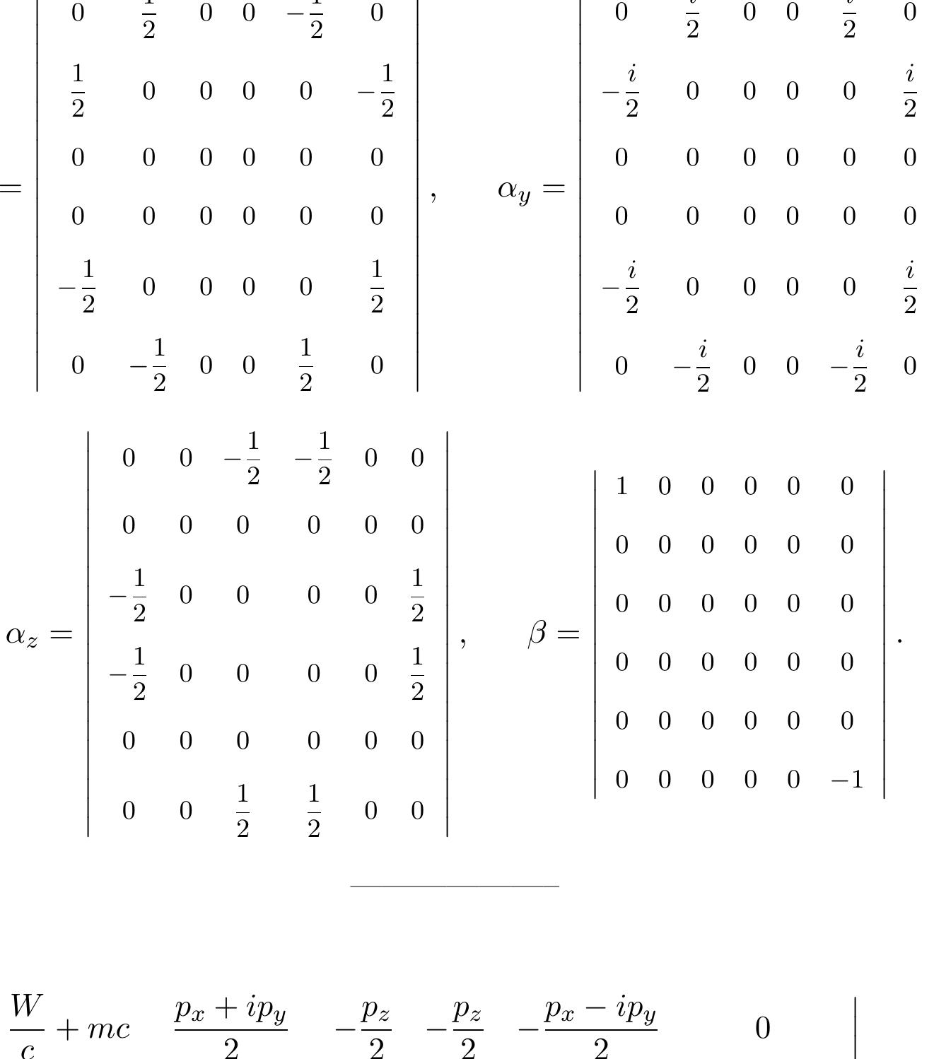


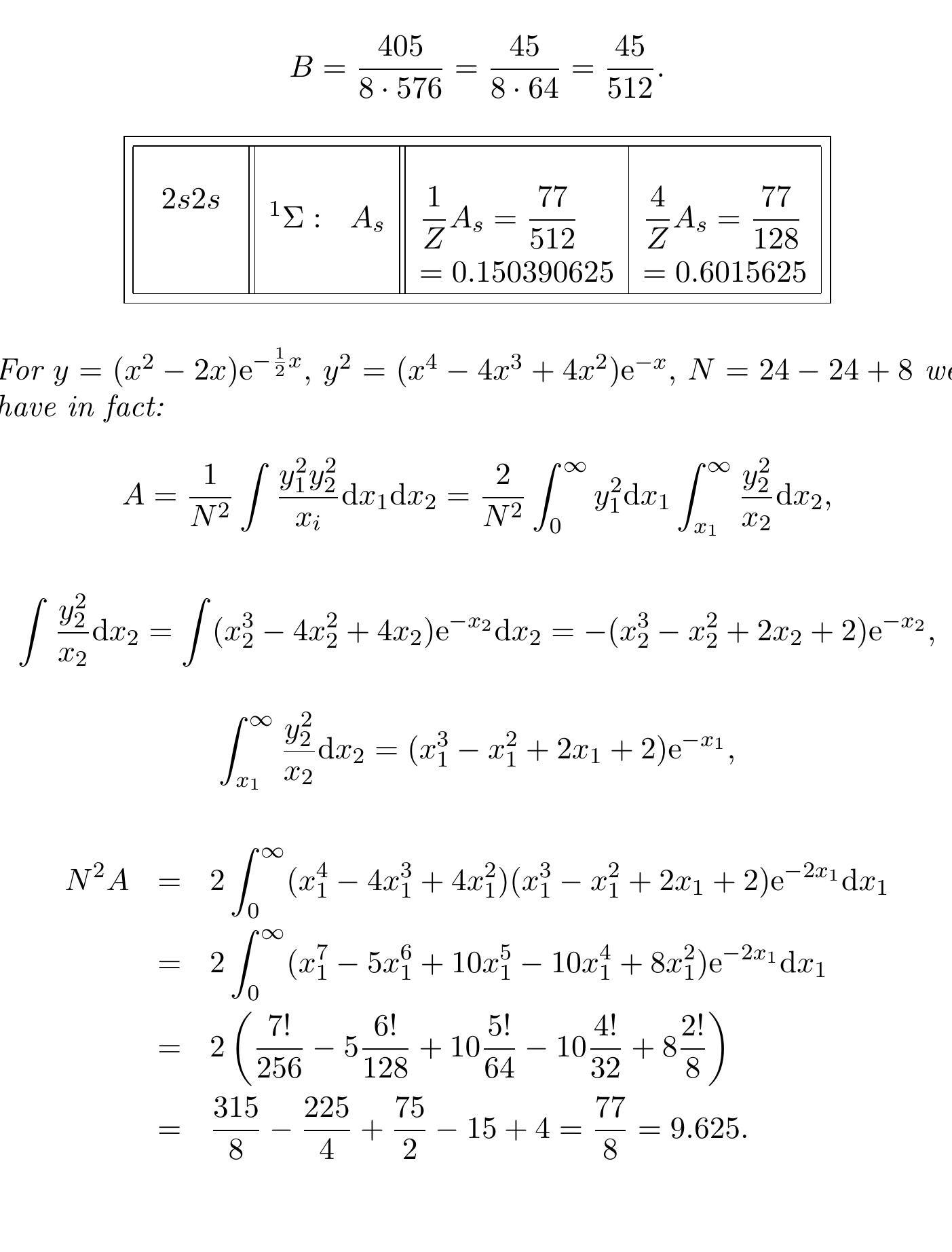


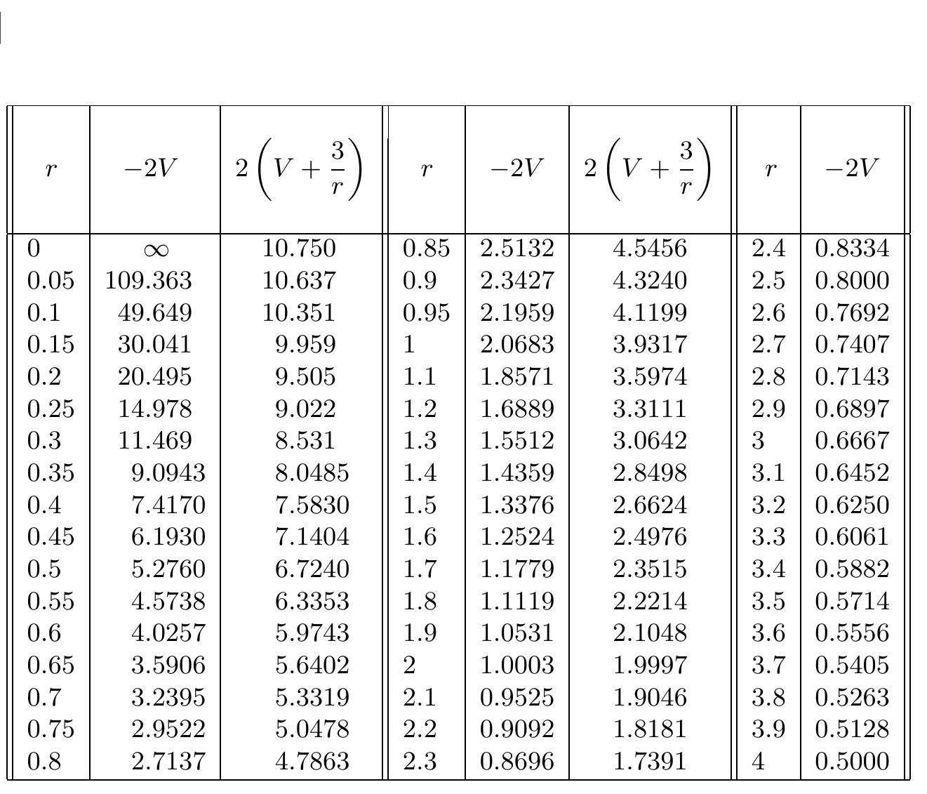


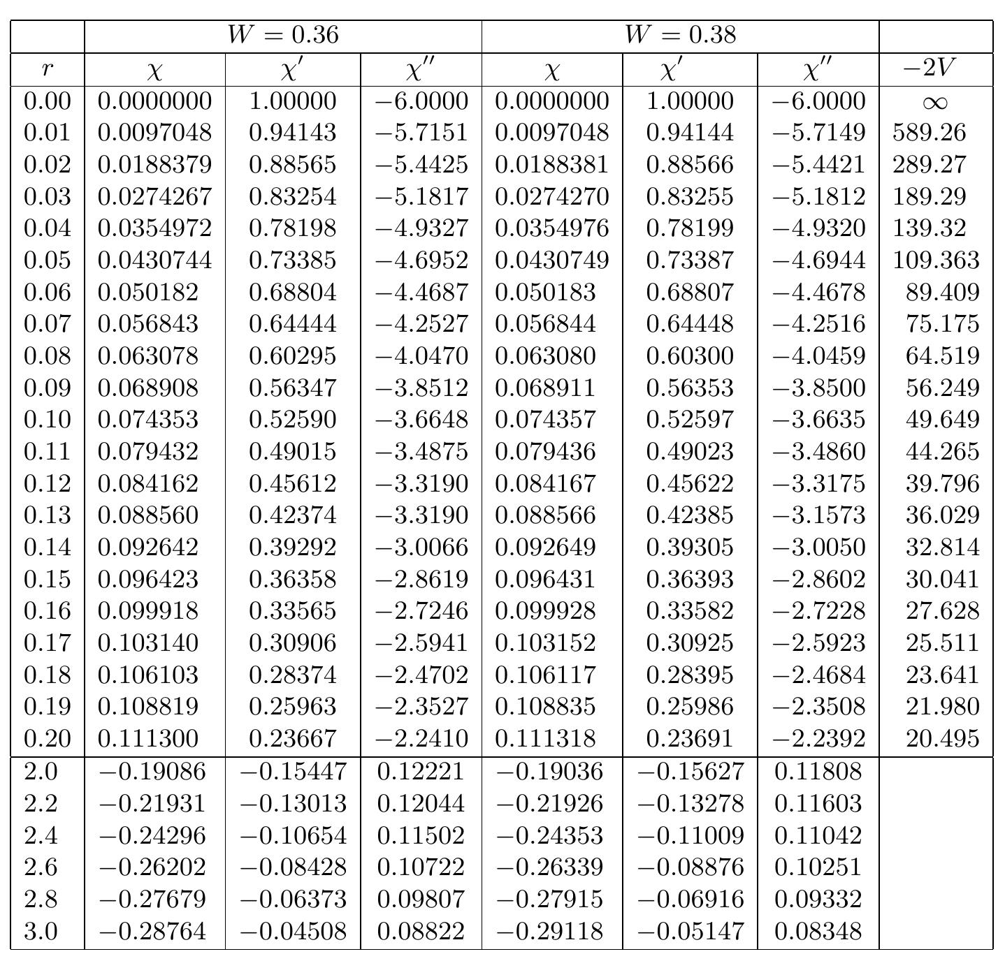


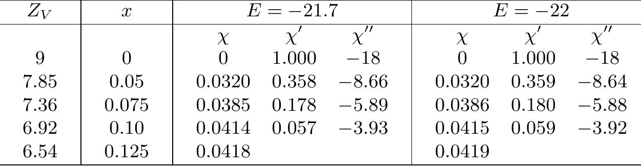


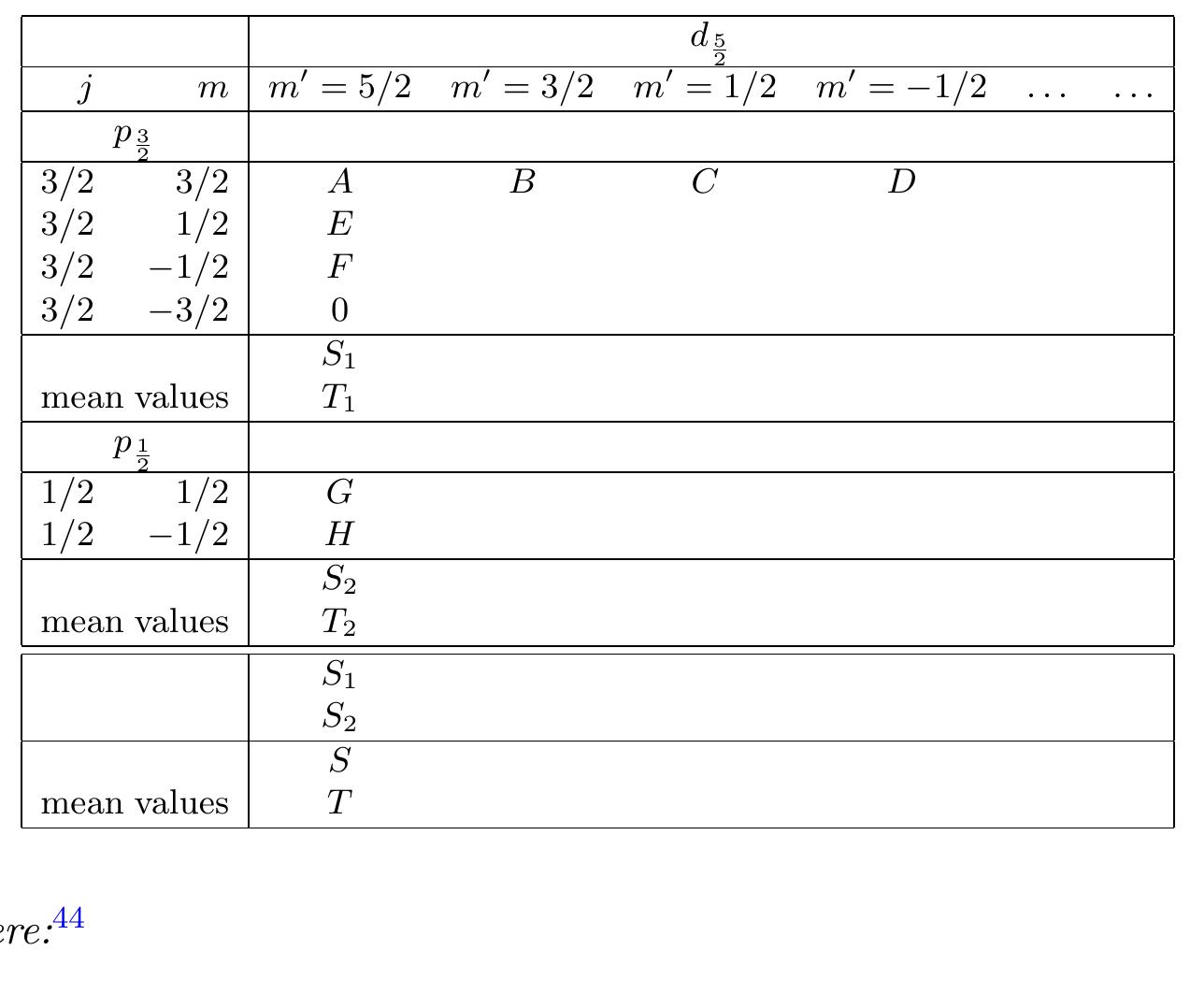


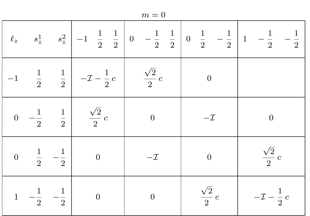


![[See equation on page 259.]](https://figures.academia-assets.com/38311747/table_026.jpg)


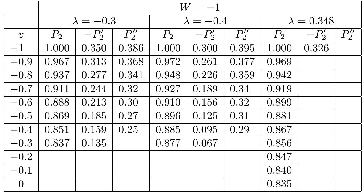


![[The footnote continues on the next page]. 3@ In the original manuscript, the following calculations appear at this point:](https://figures.academia-assets.com/38311747/figure_306.jpg)


![7.3.5.2 Zeroth approximation C=0; P?Vp = P®Vy; P = constant, P’ = constant. k= PUP, t= Py] P-](https://figures.academia-assets.com/38311747/figure_354.jpg)