
Machine Learning is a subset of artificial intelligence that focuses on the development of computer software or programs that access data to learn from them and make predictions.

R language is being used in building machine learning models due to its flexibility, efficient packages and the ability to perform deep learning models with integration to the cloud. Being an open-source language, it offers multiple packages. Following are some famous R packages widely used in industry.
1. data.table
data.table package is a enhanced version of data.frame package and is designed for high-performance. It is known for its memory efficiency and ability to perform complex data manipulations at high speed. Some key features of data.table are:
- Fast file reading and writing
- Scalable data aggregation with parallelism support
- Feature-rich data reshaping
- Simplified syntax for subsetting and merging data
install.packages("data.table")
library(data.table)

iris_dt <- as.data.table(iris)

result <- iris_dt[Species == "setosa" & Sepal.Length > 5][1:5]
result
Output:

2. Dplyr
Dplyr package is one of the most widely used data manipulation tools in R. It provides easy to implement and consistent set of functions to perform data transformations. The key functions in dplyr are:
- select(): Choose columns by name
- filter(): Subset rows based on conditions
- arrange(): Sort rows by column values
- mutate(): Add new variables
Select and Mutate Functions :
install.packages("dplyr")  # Run only once
library(dplyr)

data("mtcars")

cat("---- Select ----\n")
selected <- dplyr::select(mtcars, mpg, cyl)
head(selected)
cat("\n------------------\n")

cat("---- Mutate ----\n")
mutated <- dplyr::mutate(mtcars, power_to_weight = hp / wt)
head(mutated)
cat("\n------------------\n")
Output:

Filter and Arrange Functions :
cat("---- Filter ----\n")
filtered <- dplyr::filter(mtcars, cyl == 6)
head(filtered)
cat("\n------------------\n")

cat("---- Arrange ----\n")
arranged <- dplyr::arrange(mtcars, desc(mpg))
head(arranged)
cat("\n------------------\n")
Output:

3. ggplot2
ggplot2 is an open-source visualization package based on the Grammar of Graphics. It is widely regarded as one of the most famous and flexible visualization libraries in R. With ggplot2 users can create a wide range of static and interactive visualizations including:
- Bar charts
- Scatter plots
- Line graphs
- Histograms
- Boxplots
The syntax is easy and visualizations are highly customizable making it go-to package for data visualization in R.
install.packages("dplyr")
install.packages("ggplot2")
library(dplyr)
library(ggplot2)

ggplot(data = mtcars,
       aes(x = hp, y = mpg,
           col = disp)) + geom_point()
Output:

4. caret
caret package (Classification and Regression Training) provides a comprehensive framework for building machine learning models in R. It includes tools for:
- Data splitting
- Preprocessing
- Feature selection
- Model training
- Model evaluation
caret supports numerous machine learning algorithms and is commonly used in industry due to its ease of use and flexibility.
install.packages("e1071")
install.packages("caTools")
install.packages("caret")

library(e1071)
library(caTools)
library(caret)

data(iris)

split <- sample.split(iris, SplitRatio = 0.7)
train_cl <- subset(iris, split == TRUE)
test_cl <- subset(iris, split == FALSE)

train_scale <- scale(train_cl[, 1:4])
test_scale <- scale(test_cl[, 1:4])

set.seed(120)
classifier_cl <- naiveBayes(Species ~ ., data = train_cl)

y_pred <- predict(classifier_cl, newdata = test_cl)

cm <- table(test_cl$Species, y_pred)
print(classifier_cl)
print(cm)
Output:
Model classifier_cl:
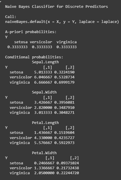
Confusion Matrix:

5. e1071
e1071 package is known for its implementation of various machine learning algorithms including support vector machines (SVM), clustering algorithms and K-Nearest Neighbors (KNN). It is widely used for classification, regression and clustering tasks.
install.packages("e1071")
install.packages("caTools")
install.packages("class")

library(e1071)
library(caTools)
library(class)

data(iris)

split <- sample.split(iris, SplitRatio = 0.7)
train_cl <- subset(iris, split == TRUE)
test_cl <- subset(iris, split == FALSE)

train_scale <- scale(train_cl[, 1:4])
test_scale <- scale(test_cl[, 1:4])

classifier_knn <- knn(train = train_scale,
                      test = test_scale,
                      cl = train_cl$Species,
                      k = 1)

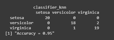
cm <- table(test_cl$Species, classifier_knn)
print(cm)

misClassError <- mean(classifier_knn != test_cl$Species)
print(paste('Accuracy =', 1 - misClassError))
Outputs:
6. XGBoost
XGBoost is a implementation of gradient boosting algorithms and is useful for large datasets. It is widely used in machine learning due to its performance and scalability. XGBoost works by bagging and boosting techniques to improve model accuracy.
install.packages("data.table")
install.packages("dplyr")
install.packages("ggplot2")
install.packages("caret")
install.packages("xgboost")
install.packages("e1071")
install.packages("cowplot")

library(data.table)
library(dplyr)
library(ggplot2)
library(caret)
library(xgboost)
library(e1071)
library(cowplot)

test[, Item_Outlet_Sales := NA]
combi = rbind(train, test)

missing_index = which(is.na(combi$Item_Weight))
for(i in missing_index){
  item = combi$Item_Identifier[i]
  combi$Item_Weight[i] = mean(combi$Item_Weight[combi$Item_Identifier == item], na.rm = T)
}

zero_index = which(combi$Item_Visibility == 0)
for(i in zero_index){
  item = combi$Item_Identifier[i]
  combi$Item_Visibility[i] = mean(combi$Item_Visibility[combi$Item_Identifier == item], na.rm = T)
}

combi[, Outlet_Size_num := ifelse(Outlet_Size == "Small", 0, ifelse(Outlet_Size == "Medium", 1, 2))]
combi[, Outlet_Location_Type_num := ifelse(Outlet_Location_Type == "Tier 3", 0, ifelse(Outlet_Location_Type == "Tier 2", 1, 2))]
combi[, c("Outlet_Size", "Outlet_Location_Type") := NULL]

ohe_1 = dummyVars("~.", data = combi[, -c("Item_Identifier", "Outlet_Establishment_Year", "Item_Type")], fullRank = T)
ohe_df = data.table(predict(ohe_1, combi[, -c("Item_Identifier", "Outlet_Establishment_Year", "Item_Type")]))
combi = cbind(combi[, "Item_Identifier"], ohe_df)

skewness(combi$Item_Visibility)
skewness(combi$price_per_unit_wt)

combi[, Item_Visibility := log(Item_Visibility + 1)]

num_vars = which(sapply(combi, is.numeric))
num_vars_names = names(num_vars)
combi_numeric = combi[, setdiff(num_vars_names, "Item_Outlet_Sales"), with = F]
prep_num = preProcess(combi_numeric, method = c("center", "scale"))
combi_numeric_norm = predict(prep_num, combi_numeric)
combi[, setdiff(num_vars_names, "Item_Outlet_Sales") := NULL]
combi = cbind(combi, combi_numeric_norm)

train = combi[1:nrow(train)]
test = combi[(nrow(train) + 1):nrow(combi)]
test[, Item_Outlet_Sales := NULL]

param_list = list(
  objective = "reg:linear",
  eta = 0.01,
  gamma = 1,
  max_depth = 6,
  subsample = 0.8,
  colsample_bytree = 0.5
)

Dtrain = xgb.DMatrix(data = as.matrix(train[, -c("Item_Identifier", "Item_Outlet_Sales")]), label = train$Item_Outlet_Sales)
Dtest = xgb.DMatrix(data = as.matrix(test[, -c("Item_Identifier")]))

set.seed(112)
xgbcv = xgb.cv(params = param_list, data = Dtrain, nrounds = 1000, nfold = 5, print_every_n = 10, early_stopping_rounds = 30, maximize = F)

xgb_model = xgb.train(data = Dtrain, params = param_list, nrounds = 428)
xgb_model
Output:

7. randomForest
Random Forest in R Programming is an ensemble learning method that builds multiple decision trees and combines them to provide more accurate predictions. It is especially useful for classification and regression tasks. Each decision tree is trained on a subset of the data and predictions are made by aggregating the results of all trees.
install.packages("caTools")
install.packages("randomForest")

library(caTools)
library(randomForest)

data(iris)

split <- sample.split(iris, SplitRatio = 0.7)
train <- subset(iris, split == "TRUE")
test <- subset(iris, split == "FALSE")

set.seed(120)
classifier_RF = randomForest(x = train[-5], y = train$Species, ntree = 500)

classifier_RF

y_pred = predict(classifier_RF, newdata = test[-5])
cm = table(test[, 5], y_pred)
cm
Outputs:
Model classifier_RF:

Confusion Matrix:
