Generative Adversarial Network (GAN)

GANs are models that generate new, realistic data by learning from existing data. Introduced by Ian Goodfellow in 2014, they enable machines to create content like images, videos and music.

They are useful because:

• Create new data similar to real world data
• Go beyond classification to generate content
• Used in art, gaming, healthcare and data science

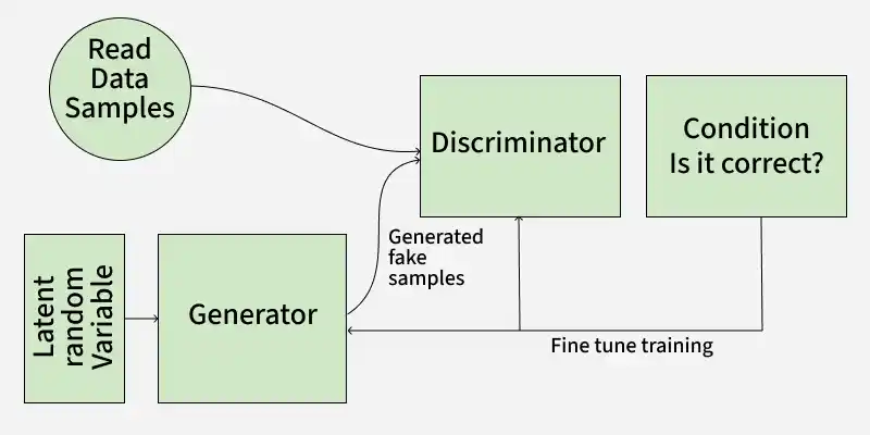
Architecture of GAN

GAN consists of two neural networks the generator and the discriminator trained adversarially, where the generator tries to fool the discriminator and the discriminator tries to distinguish real from fake data.

1. Generator Model

The generator is a deep neural network that takes random noise as input to generate realistic data samples like images or text. It learns the underlying data patterns by adjusting its internal parameters during training through backpropagation. Its objective is to produce samples that the discriminator classifies as real.

Generator Loss Function: The generator tries to minimize this loss:

J_{G} = -\frac{1}{m} \Sigma^m _{i=1} log D(G(z_{i}))

where

• J_Gmeasure how well the generator is fooling the discriminator.
• G(z_i) is the generated sample from random noise z_i
• D(G(z_i)) is the discriminator’s estimated probability that the generated sample is real.

The generator aims to maximize D(G(z_i)) meaning it wants the discriminator to classify its fake data as real (probability close to 1).

2. Discriminator Model

The discriminator is a binary classifier that distinguishes real data from generated samples. Through training, it refines its parameters to improve detection of fake data and when working with images, it uses convolutional layers to extract features and enhance classification accuracy.

Discriminator Loss Function: The discriminator tries to minimize this loss:

J_{D} = -\frac{1}{m} \Sigma_{i=1}^m log\; D(x_{i}) - \frac{1}{m}\Sigma_{i=1}^m log(1 - D(G(z_{i}))

• J_D measures how well the discriminator classifies real and fake samples.
• x_{i} is a real data sample.
• G(z_{i}) is a fake sample from the generator.
• D(x_{i}) is the discriminator’s probability that x_{i} is real.
• D(G(z_{i})) is the discriminator’s probability that the fake sample is real.

The discriminator wants to correctly classify real data as real (maximize log D(x_{i}) and fake data as fake (maximize log(1 - D(G(z_{i})))

MinMax Loss

GANs are trained using a MinMax Loss between the generator and discriminator:

min_{G}\;max_{D}(G,D) = [\mathbb{E}_{x∼p_{data}}[log\;D(x)] + \mathbb{E}_{z∼p_{z}(z)}[log(1 - D(g(z)))]

where:

• G is generator network and is D is the discriminator network
• p_{data}(x) = true data distribution
• p_z(z) = distribution of random noise (usually normal or uniform)
• D(x) = discriminator’s estimate of real data
• D(G(z)) = discriminator’s estimate of generated data

The generator tries to minimize this loss (to fool the discriminator) and the discriminator tries to maximize it (to detect fakes accurately).

Working of GAN

GAN train by having two networks the Generator (G) and the Discriminator (D) compete and improve together. Here's the step-by-step process

1. Generator's First Move

The generator starts with a random noise vector like random numbers. It uses this noise as a starting point to create a fake data sample such as a generated image. The generator’s internal layers transform this noise into something that looks like real data.

2. Discriminator's Turn

The discriminator receives two types of data:

• Real samples from the actual training dataset.
• Fake samples created by the generator.

D's job is to analyze each input and find whether it's real data or something G cooked up. It outputs a probability score between 0 and 1. A score of 1 shows the data is likely real and 0 suggests it's fake.

3. Adversarial Learning

• If the discriminator correctly classifies real and fake data it gets better at its job.
• If the generator fools the discriminator by creating realistic fake data, it receives a positive update and the discriminator is penalized for making a wrong decision.

4. Generator's Improvement

• Each time the discriminator mistakes fake data for real, the generator learns from this success.
• Through many iterations, the generator improves and creates more convincing fake samples.

5. Discriminator's Adaptation

• The discriminator also learns continuously by updating itself to better spot fake data.
• This constant back-and-forth makes both networks stronger over time.

6. Training Progression

• As training continues, the generator becomes highly proficient at producing realistic data.
• Ideally, the generator improves to the point where the discriminator finds it difficult to distinguish real from generated data, although in practice GAN training can be unstable and may not always reach this balance.
• At this point, the generator can produce high quality synthetic data that can be used for different applications.

Types of GAN

There are several types of GANs each designed for different purposes. Here are some important types:

1. Vanilla GAN

Vanilla GAN is the simplest type of GAN. It consists of:

• A generator and a discriminator both are built using multi-layer perceptrons (MLPs).
• The model optimizes its mathematical formulation using stochastic gradient descent (SGD).

While foundational, Vanilla GAN can face problems like:

• Generator produces limited types of outputs repeatedly.
• Generator and discriminator may not improve smoothly.

2. Conditional GAN (CGAN)

Conditional GAN (CGAN) adds an additional conditional parameter to guide the generation process. Instead of generating data randomly they allow the model to produce specific types of outputs.

Working of CGANs:

• A conditional variable (y) is fed into both the generator and the discriminator.
• This ensures that the generator creates data corresponding to the given condition (e.g generating images of specific objects).
• The discriminator also receives the labels to help distinguish between real and fake data.

Example: Instead of generating any random image, CGAN can generate a specific object like a dog or a cat based on the label.

3. Deep Convolutional GAN (DCGAN)

Deep Convolutional GAN (DCGAN) are among the most popular types of GANs used for image generation.

They are important because they:

• Uses Convolutional Neural Networks (CNNs) instead of simple multi-layer perceptrons (MLPs).
• Max pooling layers are replaced with convolutional stride helps in making the model more efficient.
• Fully connected layers are removed, which allows for better spatial understanding of images.

DCGANs are successful because they generate high-quality, realistic images.

4. Laplacian Pyramid GAN (LAPGAN)

Laplacian Pyramid GAN (LAPGAN) is designed to generate ultra-high-quality images by using a multi-resolution approach.

Working of LAPGAN:

• Uses multiple generator-discriminator pairs at different levels of the Laplacian pyramid.
• Images are first down sampled at each layer of the pyramid and upscaled again using Conditional GAN (CGAN).
• This process allows the image to gradually refine details and helps in reducing noise and improving clarity.

Due to its ability to generate highly detailed images, LAPGAN is considered a superior approach for photorealistic image generation.

5. Super Resolution GAN (SRGAN)

Super-Resolution GAN (SRGAN) is designed to increase the resolution of low-quality images while preserving details.

Working of SRGAN:

• Uses a deep neural network combined with an adversarial loss function.
• Enhances low-resolution images by adding finer details helps in making them appear sharper and more realistic.
• Helps to reduce common image upscaling errors such as blurriness and pixelation.

Implementation

Generative Adversarial Networks (GAN) can generate realistic images by learning from existing image datasets. Here we will be implementing a GAN trained on the CIFAR-10 dataset using PyTorch.

Step 1: Importing Required Libraries

We will be using Pytorch, Torchvision, Matplotlib and Numpy libraries for this. Set the device to GPU if available otherwise use CPU.

import torch
import torch.nn as nn
import torch.optim as optim
import torchvision
from torchvision import datasets, transforms
import matplotlib.pyplot as plt
import numpy as np

device = torch.device('cuda' if torch.cuda.is_available() else 'cpu')

Step 2: Defining Image Transformations

We use PyTorch’s transforms to convert images to tensors and normalize pixel values between -1 and 1 for better training stability.

transform = transforms.Compose([
    transforms.ToTensor(),
    transforms.Normalize((0.5, 0.5, 0.5), (0.5, 0.5, 0.5))
])

Step 3: Loading the CIFAR-10 Dataset

Download and load the CIFAR-10 dataset with defined transformations. Use a DataLoader to process the dataset in mini-batches of size 32 and shuffle the data.

train_dataset = datasets.CIFAR10(root='./data',\
              train=True, download=True, transform=transform)
dataloader = torch.utils.data.DataLoader(train_dataset, \
                                batch_size=32, shuffle=True)

Step 4: Defining GAN Hyperparameters

Set important training parameters:

• latent_dim: Dimensionality of the noise vector.
• lr: Learning rate of the optimizer.
• beta1, beta2: Beta parameters for Adam optimizer (e.g 0.5, 0.999)
• num_epochs: Number of times the entire dataset will be processed (e.g 10)

latent_dim = 100
lr = 0.0002
beta1 = 0.5
beta2 = 0.999
num_epochs = 10

Step 5: Building the Generator

Create a neural network that converts random noise into images. Use transpose convolutional layers, batch normalization and ReLU activations. The final layer uses Tanh activation to scale outputs to the range [-1, 1].

• nn.Linear(latent_dim, 128 * 8 * 8): Defines a fully connected layer that projects the noise vector into a higher dimensional feature space.
• nn.Upsample(scale_factor=2): Doubles the spatial resolution of the feature maps by upsampling.
• nn.Conv2d(128, 128, kernel_size=3, padding=1): Applies a convolutional layer keeping the number of channels the same to refine features.

class Generator(nn.Module):
    def __init__(self, latent_dim):
        super(Generator, self).__init__()

        self.model = nn.Sequential(
            nn.Linear(latent_dim, 128 * 8 * 8),
            nn.ReLU(),
            nn.Unflatten(1, (128, 8, 8)),
            nn.Upsample(scale_factor=2),
            nn.Conv2d(128, 128, kernel_size=3, padding=1),
            nn.BatchNorm2d(128, momentum=0.78),
            nn.ReLU(),
            nn.Upsample(scale_factor=2),
            nn.Conv2d(128, 64, kernel_size=3, padding=1),
            nn.BatchNorm2d(64, momentum=0.78),
            nn.ReLU(),
            nn.Conv2d(64, 3, kernel_size=3, padding=1),
            nn.Tanh()
        )

    def forward(self, z):
        img = self.model(z)
        return img

Step 6: Building the Discriminator

Create a binary classifier network that distinguishes real from fake images. Use convolutional layers, batch normalization, dropout, LeakyReLU activation and a Sigmoid output layer to give a probability between 0 and 1.

• nn.Conv2d(32, 64, kernel_size=3, stride=2, padding=1): Second convolutional layer increasing channels to 64, downsampling further.
• nn.BatchNorm2d(256, momentum=0.8): Batch normalization for 256 feature maps with momentum 0.8.

class Discriminator(nn.Module):
    def __init__(self):
        super(Discriminator, self).__init__()

        self.model = nn.Sequential(
        nn.Conv2d(3, 32, kernel_size=3, stride=2, padding=1),
        nn.LeakyReLU(0.2),
        nn.Dropout(0.25),
        nn.Conv2d(32, 64, kernel_size=3, stride=2, padding=1),
        nn.ZeroPad2d((0, 1, 0, 1)),
        nn.BatchNorm2d(64, momentum=0.82),
        nn.LeakyReLU(0.25),
        nn.Dropout(0.25),
        nn.Conv2d(64, 128, kernel_size=3, stride=2, padding=1),
        nn.BatchNorm2d(128, momentum=0.82),
        nn.LeakyReLU(0.2),
        nn.Dropout(0.25),
        nn.Conv2d(128, 256, kernel_size=3, stride=1, padding=1),
        nn.BatchNorm2d(256, momentum=0.8),
        nn.LeakyReLU(0.25),
        nn.Dropout(0.25),
        nn.Flatten(),
        nn.Linear(256 * 5 * 5, 1),
        nn.Sigmoid()
    )

    def forward(self, img):
        validity = self.model(img)
        return validity

Step 7: Initializing GAN Components

• Generator and Discriminator are initialized on the available device (GPU or CPU).
• Binary Cross-Entropy (BCE) Loss is chosen as the loss function.
• Adam optimizers are defined separately for the generator and discriminator with specified learning rates and betas.

generator = Generator(latent_dim).to(device)
discriminator = Discriminator().to(device)

adversarial_loss = nn.BCELoss()

optimizer_G = optim.Adam(generator.parameters()\
                         , lr=lr, betas=(beta1, beta2))
optimizer_D = optim.Adam(discriminator.parameters()\
                         , lr=lr, betas=(beta1, beta2))

Step 8: Training the GAN

Train the discriminator on real and fake images, then update the generator to improve its fake image quality. Track losses and visualize generated images after each epoch.

• valid = torch.ones(real_images.size(0), 1, device=device): Create a tensor of ones representing real labels for the discriminator.
• fake = torch.zeros(real_images.size(0), 1, device=device): Create a tensor of zeros representing fake labels for the discriminator.
• z = torch.randn(real_images.size(0), latent_dim, device=device): Generate random noise vectors as input for the generator.
• g_loss = adversarial_loss(discriminator(gen_images), valid): Calculate generator loss based on the discriminator classifying fake images as real.
• grid = torchvision.utils.make_grid(generated, nrow=4, normalize=True): Arrange generated images into a grid for display, normalizing pixel values.

for epoch in range(num_epochs):
    for i, batch in enumerate(dataloader):
       
        real_images = batch[0].to(device) 
       
        valid = torch.ones(real_images.size(0), 1, device=device)
        fake = torch.zeros(real_images.size(0), 1, device=device)
       
        real_images = real_images.to(device)

        optimizer_D.zero_grad()
       
        z = torch.randn(real_images.size(0), latent_dim, device=device)
      
        fake_images = generator(z)

        real_loss = adversarial_loss(discriminator\
                                     (real_images), valid)
        fake_loss = adversarial_loss(discriminator\
                                     (fake_images.detach()), fake)
        d_loss = (real_loss + fake_loss) / 2
    
        d_loss.backward()
        optimizer_D.step()

        optimizer_G.zero_grad()
      
        gen_images = generator(z)
        
        g_loss = adversarial_loss(discriminator(gen_images), valid)
        g_loss.backward()
        optimizer_G.step()
       
        if (i + 1) % 100 == 0:
            print(
                f"Epoch [{epoch+1}/{num_epochs}]\
                        Batch {i+1}/{len(dataloader)} "
                f"Discriminator Loss: {d_loss.item():.4f} "
                f"Generator Loss: {g_loss.item():.4f}"
            )
    if (epoch + 1) % 10 == 0:
        with torch.no_grad():
            z = torch.randn(16, latent_dim, device=device)
            generated = generator(z).detach().cpu()
            grid = torchvision.utils.make_grid(generated,\
                                        nrow=4, normalize=True)
            plt.imshow(np.transpose(grid, (1, 2, 0)))
            plt.axis("off")
            plt.show()

Output:

By following these steps we successfully implemented and trained a GAN that learns to generate realistic CIFAR-10 images through adversarial training.

You can download source code from here.

Applications

• Generate realistic images, avatars and high-resolution visuals by learning data patterns, widely used in art, gaming and design.
• Transform images across domains (e.g., day to night, sketch to real) while preserving important features.
• Create images from text descriptions, enabling AI-based art and automated content generation.
• Generate synthetic data to enhance model training, improving robustness when real data is limited.
• Upscale low-resolution images to improve clarity, useful in medical imaging, satellite imagery and video enhancement.

Advantages

• Produce new, synthetic data resembling real data distributions which is useful for augmentation, anomaly detection and creative tasks.
• Can generate photorealistic images, videos, music and other media with high quality.
• They don’t require labeled data helps in making them effective in scenarios where labeling is expensive or difficult.
• Can be applied across many tasks including image synthesis, text-to-image generation, style transfer, anomaly detection and more.