Data Science Interview Questions and Answers

In this Data Science interview questions guide, you will explore interview questions for Data Science for beginners and experienced professionals. Here you will find the frequently asked questions during the data science interview. Practicing all the questions below will help you explore your career as a data scientist.

1. What is the difference between Data Science and Data Analytics?

Data Science and Data Analytics both involve working with data to support decision-making, but they have different objectives.

Data Science

Data Science is an interdisciplinary field that combines statistics, programming, machine learning, and domain knowledge to extract insights from data.
It works with both structured and unstructured data.
It involves the complete data lifecycle, including data collection, cleaning, analysis, visualization, model building, and deployment.
It focuses on predictive and prescriptive analytics using machine learning and AI techniques.
It is widely used for recommendation systems, fraud detection, forecasting, and predictive modeling.
Goal: Discover patterns and build intelligent models that can make predictions or automate decisions.

Data Analytics

Data Analytics focuses on examining historical data to identify patterns, trends, and business insights.
It primarily works with structured data from databases, spreadsheets, and data warehouses.
It involves data cleaning, querying, visualization, and reporting.
It focuses mainly on descriptive and diagnostic analytics to understand what happened and why.
It is widely used for business reporting, performance monitoring, customer behavior analysis, and KPI tracking.
Goal: Analyze existing data to support informed business decisions.

2. What are the different types of data used in Data Science?

Structured Data: Data organized in a fixed format like rows and columns (e.g., data in a SQL database or Excel sheet).
Semi-Structured Data: Data that doesn't fit neatly into tables but has some organizational structure (e.g., JSON, XML files).
Unstructured Data: Data with no predefined format (e.g., images, audio, video, free-form text).

3. What is the Data Science Lifecycle?

The Data Science Lifecycle is the step-by-step process followed to solve a problem using data:

Problem Definition: Understanding the business problem and defining the goal.
Data Collection: Gathering data from databases, APIs, files, or web scraping.
Data Cleaning & Preprocessing: Handling missing values, duplicates, and inconsistent formats.
Exploratory Data Analysis (EDA): Understanding patterns and relationships using statistics and visualization.
Feature Engineering: Creating or transforming variables to improve model performance.
Model Building: Applying ML or statistical models to the data.
Model Evaluation: Testing performance using appropriate metrics.
Deployment: Putting the model into production.
Monitoring & Maintenance: Tracking model performance over time and retraining when needed.

4. What is the difference between Data Science, Machine Learning, and Artificial Intelligence?

Data Science, Machine Learning (ML), and Artificial Intelligence (AI) are closely related fields but serve different purposes.

Data Science

Data Science is an interdisciplinary field that combines statistics, programming, domain knowledge, and machine learning to extract meaningful insights from data.
It involves the complete data lifecycle, including data collection, cleaning, analysis, visualization, and model building.
It works with both structured and unstructured data.
Machine Learning is one of the many tools used in Data Science.
Goal: Transform raw data into actionable insights and support data-driven decision-making.

Machine Learning (ML)

Machine Learning is a subset of Artificial Intelligence that enables systems to learn from data without being explicitly programmed.
It uses algorithms to identify patterns and make predictions or decisions.
The model improves its performance as it is exposed to more data.
It includes supervised, unsupervised, semi-supervised, and reinforcement learning techniques.
Goal: Build models that can learn from data and make accurate predictions or decisions.

Artificial Intelligence (AI)

Artificial Intelligence is the broader field of creating systems that can mimic human intelligence.
It includes reasoning, learning, problem-solving, planning, perception, and decision-making.
AI encompasses Machine Learning, Deep Learning, expert systems, robotics, and natural language processing.
It aims to automate intelligent tasks that typically require human intelligence.
Goal: Develop intelligent systems capable of performing complex cognitive tasks.

5. What is the difference between Data Science and Data Engineering?

Data Science and Data Engineering are complementary fields in the data ecosystem. Data Engineering focuses on building and maintaining the infrastructure required to collect, process, and store data, whereas Data Science focuses on analyzing that data to extract insights and build predictive models.

Data Science

Data Science focuses on extracting meaningful insights from data using statistics, machine learning, and data visualization.
It involves data exploration, feature engineering, model building, evaluation, and deployment.
It works with both structured and unstructured data.
It helps organizations make data-driven decisions and build predictive models.
Common tools include Python, R, TensorFlow, Scikit-learn, Pandas, and Jupyter Notebook.
Goal: Analyze data and develop models that generate insights and predictions.

Data Engineering

Data Engineering focuses on designing, building, and maintaining data pipelines and infrastructure.
It is responsible for collecting, transforming, storing, and processing large volumes of data.
It ensures that data is clean, reliable, and readily available for analytics and machine learning.
It works with distributed systems, databases, cloud platforms, and ETL/ELT pipelines.
Common tools include Apache Spark, Hadoop, Kafka, Airflow, SQL, Snowflake, and cloud services such as AWS, Azure, or Google Cloud

6. What is Python and why is it widely used in Data Science?

Python is a high-level, general-purpose programming language known for its simple, readable syntax. It has become the dominant language in Data Science for several reasons:

Rich ecosystem of libraries: NumPy and Pandas for data handling, Matplotlib/Seaborn for visualization, Scikit-learn for classical ML, and TensorFlow/PyTorch for deep learning — covering the entire DS workflow.
Ease of learning and experimentation: Simple syntax lets data scientists focus on logic rather than boilerplate code, speeding up prototyping.
Strong community and integration: Python connects easily with SQL databases, big data tools (Spark), cloud platforms, and APIs.
Versatility: The same language can handle data cleaning, statistical analysis, model building, and deployment.

7. What is the difference between a List and a Tuple in Python?

Lists and Tuples are both ordered collections in Python, but they differ in mutability and use case:

List: Mutable — elements can be added, removed, or changed after creation. Defined using square brackets: [1, 2, 3].
Tuple: Immutable — once created, elements cannot be changed. Defined using parentheses: (1, 2, 3).

8. What is NumPy and why is it faster than regular Python lists?

NumPy (Numerical Python) is a library that provides support for large, multi-dimensional arrays and matrices, along with a collection of mathematical functions to operate on them efficiently. It is one of the foundational libraries for numerical computing in Data Science.

Contiguous memory storage: NumPy arrays store elements in a single, contiguous block of memory, unlike Python lists which store references to scattered objects. This makes NumPy operations far more cache-efficient.
Vectorized operations: NumPy performs operations on entire arrays at once using optimized, pre-compiled C code under the hood, avoiding the overhead of Python's loop interpretation.
Fixed data type: All elements in a NumPy array share the same data type, which avoids the type-checking overhead Python lists incur for each element.

9. What is Pandas and what are its main data structures?

Pandas is a Python library built on top of NumPy, designed specifically for data manipulation and analysis. It introduces two core data structures:

Series: A one-dimensional labeled array, similar to a single column in a spreadsheet. Each element has an associated index label.
DataFrame: A two-dimensional labeled data structure, similar to a table in a database or an Excel sheet, where each column is essentially a Series and all columns share a common index..

10. How do you handle missing values in Pandas?

Handling missing values is a critical step in data cleaning. Pandas provides several approaches depending on the situation:

1. Detection:

isnull()/notnull() — return boolean masks indicating where values are missing.

2. Removal:

dropna() — removes rows or columns containing missing values. Useful when missing data is minimal and random.

3. Imputation:

fillna(value) — replaces missing values with a specific value, or with statistical measures like mean, median (for numerical data), or mode (for categorical data).
Forward Fill (ffill) / Backward Fill (bfill) — propagates the previous or next valid value forward/backward, especially useful in time series data where order matters.

4. Prediction-based imputation:

Missing values can also be predicted using a model trained on the other available features, which is more accurate than simple mean/median imputation but computationally expensive.

11. What is SQL, and what does it stand for?

SQL stands for Structured Query Language , a domain-specific language used to communicate with and manage relational databases.

It allows users to define database structures (DDL), manipulate data (DML), control access (DCL), and query data (DQL) using a declarative syntax.
You specify what data you want, not how to retrieve it; the database engine determines the most efficient execution plan.

12. What is the difference between SQL and NoSQL databases?

SQL and NoSQL databases differ fundamentally in how they structure and scale data:

SQL Databases

SQL (Structured Query Language) databases store data in tables consisting of rows and columns.
They follow a fixed schema, meaning the structure of the data must be defined before storing it.
They support ACID (Atomicity, Consistency, Isolation, Durability) properties, ensuring reliable transactions.
They are well suited for applications requiring complex queries and strong data consistency.
Common SQL databases include MySQL, PostgreSQL, Oracle Database, and Microsoft SQL Server.
Goal: Store and manage structured data with strong consistency and reliable transactions.

NoSQL Databases

NoSQL (Not Only SQL) databases store data using flexible models such as document, key-value, column-family, or graph.
They support dynamic schemas, allowing data structures to evolve without predefined tables.
They are designed for horizontal scaling and handling large volumes of distributed data.
They often prioritize high availability and scalability over strict consistency, depending on the database type.
Common NoSQL databases include MongoDB, Cassandra, Redis, and Neo4j.
Goal: Efficiently manage large-scale structured, semi-structured, and unstructured data.

13. What are the main components (clauses) of a SQL query and in what order do they execute?

Logical execution order:

FROM – identifies the source table(s)
WHERE – filters individual rows based on a condition
GROUP BY – groups the filtered rows
HAVING – filters the grouped results
SELECT – picks the columns/expressions to return
ORDER BY – sorts the final result
LIMIT – restricts the number of rows returned

This is exactly why you can use an aggregate function like COUNT(*) inside HAVING but not inside WHERE — by the time WHERE runs, grouping hasn't happened yet, so there's nothing to aggregate.

14. What is the difference between a Primary Key and a Foreign Key?

Primary Key: A column (or combination of columns) that uniquely identifies each row in its own table. It cannot contain NULL values and must be unique across all rows. A table can have only one primary key.
Foreign Key: A column in one table that references the primary key of another table, establishing a relationship between the two. Unlike a primary key, it can contain duplicate values and, in most databases, can be NULL (if the relationship is optional). A table can have multiple foreign keys.

Example: In an Orders table, order_id would be the primary key (uniquely identifies each order), while customer_id would be a foreign key referencing the Customers table — enforcing that every order must belong to a valid, existing customer.

15. What is the difference between the WHERE and HAVING clause?

Both clauses filter data, but at different stages of query execution:

WHERE: filters individual rows before any grouping occurs. It cannot use aggregate functions like SUM() or COUNT().
HAVING: filters groups of rows after GROUP BY has aggregated them. It is specifically designed to work with aggregate functions.

16. What is the difference between INNER JOIN, LEFT JOIN, RIGHT JOIN, and FULL JOIN?

JOINs combine rows from two or more tables based on a related column, but they differ in how they treat unmatched rows:

INNER JOIN: Returns only the rows that have matching values in both tables. Non-matching rows from either table are excluded entirely.
LEFT JOIN: Returns all rows from the left table, along with matched rows from the right table. If there's no match, the right table's columns are filled with NULL.
RIGHT JOIN: The mirror of LEFT JOIN — returns all rows from the right table, with unmatched left table columns filled as NULL.
FULL JOIN: Returns all rows from both tables. Where there's no match on either side, the missing side's columns are filled with NULL.

17. What are Window Functions and how do they differ from Aggregate Functions?

A window function performs a calculation across a set of rows related to the current row defined by an OVER() clause without collapsing those rows into a single output. This is the key distinction from regular aggregate functions.

Aggregate function: Collapses multiple rows into one summary row per group.
Window function: Keeps every original row intact while still computing the aggregate value relative to a "window" of related rows.

Example: SUM() with GROUP BY is aggregate function and SUM() OVER(PARTITION BY ) is window function.

18. What's the difference between `COUNT(*)`, `COUNT(1)`, and `COUNT(column_name)` ?

COUNT(*): Counts all rows, including those with NULL values in any column.
COUNT(1): Functionally identical to COUNT(*) counts all rows. The 1 is just a constant expression evaluated for every row; it does not reference any actual column.
COUNT(column_name): Counts only the rows where that specific column is NOT NULL, NULL values are excluded from the count.

19. What is the difference between a JOIN and a SUBQUERY, and when would you use each?

JOIN: Combines columns from two or more tables into a single result set based on a related column, evaluated together by the query optimizer. Generally more efficient for retrieving combined data from multiple tables, especially with proper indexing.
SUBQUERY: A query nested inside another query (in WHERE, SELECT, or FROM), used to compute an intermediate value or filter condition that the outer query then uses.

When to use JOIN: When you need actual columns from multiple tables combined into one output . e.g., "list all orders along with customer names."

When to use SUBQUERY: When you only need a value or set of values to filter the outer query, not the underlying table's columns . e.g., "find customers who spent more than the average order amount."

20. What is a CTE (Common Table Expression) and how is it different from a Subquery?

A CTE is a temporary, named result set defined using the WITH clause, which exists only for the duration of the query. It behaves like a subquery but with better readability and additional capabilities.

Key advantages over subqueries:

Readability: Breaking a complex query into named, logical steps makes it far easier to read and debug than deeply nested subqueries.
Reusability: A CTE can be referenced multiple times within the same query, whereas a subquery must be rewritten each time.
Recursion: CTEs support recursive queries (using WITH RECURSIVE), which subqueries cannot do — essential for traversing hierarchical data like an organizational chart or a category tree.

21. What are Indexes in SQL and how do they improve performance?

An Index is a database structure (commonly a B-Tree) that improves the speed of data retrieval by allowing the database engine to locate rows without scanning the entire table similar to how a book's index lets you jump directly to a topic instead of reading every page.

How it helps: Without an index, a query with a WHERE condition triggers a full table scan, checking every row. With an index on that column, the database can use the index structure to jump almost directly to matching rows, drastically reducing lookup time — especially significant on large tables.

Trade-offs:

Faster reads: Significantly speeds up SELECT queries with WHERE, JOIN, or ORDER BY on indexed columns.
Slower writes: Every INSERT, UPDATE, or DELETE must also update the index, adding overhead.
Storage cost: Indexes consume additional disk space.

22. What are ACID properties in DBMS?

ACID is a set of properties that guarantee reliable processing of database transactions, especially important in systems handling financial or critical data:

Atomicity: A transaction is treated as a single, indivisible unit — either all its operations complete successfully, or none of them do. If any part fails, the entire transaction is rolled back.
Consistency: A transaction takes the database from one valid state to another, ensuring all defined rules (constraints, triggers) are maintained.
Isolation: Concurrent transactions execute as if they were run sequentially, preventing one transaction's intermediate state from affecting another.
Durability: Once a transaction is committed, its changes are permanent and survive even a system crash or power failure.

Example: In a bank transfer, atomicity ensures that money is either fully deducted from one account and added to another, or neither happens at all — never a partial transfer.

23. What is the difference between Normalization and Denormalization?

Normalization and Denormalization are database design techniques used to organize data.

Normalization

Normalization is the process of organizing data into multiple related tables to eliminate redundancy.
It reduces data duplication and improves data consistency.
It ensures that each piece of information is stored only once.
It involves applying normal forms such as 1NF, 2NF, 3NF, and BCNF.
It may require multiple table joins, which can slow down complex queries.
Goal: Minimize redundancy and maintain data integrity.

Denormalization

Denormalization is the process of combining related tables by introducing controlled redundancy.
It reduces the need for complex joins, improving query performance.
It increases data duplication, which can lead to higher storage requirements.
It is commonly used in data warehouses and read-intensive applications.
Updating data may become more complex because the same information can exist in multiple places.
Goal: Improve query performance and reduce query execution time.

24. What are Views and Stored Procedures in SQL?

View: A virtual table defined by a saved SQL query. It doesn't store data physically every time it's queried, the underlying query runs fresh. Views are used to simplify repeated complex queries and to restrict access to sensitive columns (e.g., exposing a view without a salary column to certain users).
Stored Procedure: A precompiled, reusable block of SQL statements stored in the database, which can accept input parameters and contain control-flow logic (loops, conditionals). Stored procedures are used to automate repetitive tasks, enforce business logic at the database level, and improve performance since they're precompiled rather than parsed each time.

25. What is Data Visualization and why is it important in Data Science?

Data Visualization is the graphical representation of data using charts, plots, and dashboards to help identify patterns, trends, and outliers that are difficult to detect from raw numbers alone.

Faster pattern recognition: The human brain processes visual information far faster than tables of numbers.
Guides EDA and feature engineering: Visualizing distributions and relationships often reveals data quality issues (outliers, skew) and hints at which features matter.
Communicates findings: Stakeholders without technical backgrounds can understand a well-designed chart far more easily than a statistical summary.

26. What are the commonly used Data Visualization libraries/tools in Python?

Matplotlib: The foundational plotting library in Python — highly flexible and customizable, but requires more code to produce polished visuals.
Seaborn: Built on top of Matplotlib, provides cleaner, statistically-oriented plots (heatmaps, violin plots, pair plots) with much less code, and integrates directly with Pandas DataFrames.
Plotly: Used for interactive, web-based visualizations where users can hover, zoom, and filter directly in the chart.
Tableau / Power BI: Business intelligence tools (outside the Python ecosystem) used to build interactive dashboards, typically used by analysts and for executive/stakeholder reporting.

27. When would you use a Bar Chart, Histogram, Box Plot, or Scatter Plot?

Bar Chart: Compares values across discrete categories (e.g., total sales by region). Best for categorical data.
Histogram: Shows the distribution/frequency of a single continuous variable by grouping values into bins (e.g., the age distribution of customers). Reveals shape, skew, and modality of data.
Box Plot: Summarizes a continuous variable's distribution using its median, quartiles, and potential outliers (via the interquartile range). Especially useful for comparing distributions across multiple categories side by side.
Scatter Plot: Plots two continuous variables against each other to visually assess their relationship commonly used to spot correlation, clusters, or non-linear patterns before formal statistical testing.

28. How would you visually detect skewness in a dataset?

Skewness (asymmetry in a data distribution) can be detected visually before even calculating the skewness statistic:

Histogram / KDE (Kernel Density Estimate) plot: If the distribution's tail stretches further to the right, the data is right-skewed (positive skew); if the tail stretches further left, it's left-skewed (negative skew). A symmetric bell shape indicates no skew.
Box Plot: If the median line inside the box sits noticeably closer to one edge, or if one whisker is much longer than the other, that's a visual sign of skewness in the same direction as the longer whisker.

29. What is a Random Variable? Explain Discrete vs Continuous Random Variables.

A Random Variable is a variable whose value is a numerical outcome of a random phenomenon the bridge between probability theory and measurable data.

Discrete Random Variable: Takes a countable set of values. Example: number of heads in 10 coin flips (0, 1, 2...10 — never 3.5).
Continuous Random Variable: Can take any value within a range, including decimals. Example: a person's height or task completion time.

30. What is Marginal Probability?

Marginal probability is simply the chance of one specific event happening, without worrying about what happens with other events.

Example: if you’re looking at the probability of it raining tomorrow, you only care about the chance of rain, not what happens with other weather conditions like wind or temperature.

31. What are the Probability Axioms?

The probability axioms are just basic rules that help us understand how probabilities work. There are three main ones:

Non-Negativity Axiom: Probabilities can't be negative. The chance of something happening is always 0 or more, never less.
Normalization Axiom: If something is certain to happen (like the sun rising tomorrow), its probability is 1. So, 1 means "definitely happening."
Additivity Axiom: If two events can't happen at the same time (like rolling a 3 or a 4 on a die), the chance of either one happening is just the sum of their individual chances.

32. What is the difference between Dependent and Independent Events in Probability?

Independent Events:

Two events are independent if one event doesn't change the likelihood of the other happening.
For example, flipping a coin twice – the first flip doesn't affect the second flip.
So, the probability of both events happening is just the product of their individual probabilities.

Dependent Events:

Two events are dependent if one event affects the likelihood of the other happening.
For example, if you draw a card from a deck and don't put it back (without replacement), the chance of drawing a second card depends on what the first card was.
The probability changes because one card was already taken out.

33. What is Conditional Probability?

Conditional probability refers to the probability of an event occurring given that another event has already occurred. Mathematically, it is defined as the probability of event A occurring, given that event B has occurred and is denoted by P(A|B). The formula for conditional probability is:

P(A|B) = \frac{P(A\cap B)}{P(B)}

where:

P(A|B) is the conditional probability of event A given event B.
P(A\cap B) is the joint probability of both events A and B occurring simultaneously.
P(B) is the probability of event B occurring.

34. What is Bayes’ Theorem and when do we use it in Data Science?

Bayes' Theorem helps us figure out the probability of an event happening based on some prior knowledge or evidence. It’s like updating our guess about something when we learn new things. The formula for Bayes' Theorem is:

P(A|B) = \frac{P(B|A) \cdot P(A)}{P(B)}

Where:

P(A|B) is the probability of event A happening, given that B has happened.
P(B|A) is the probability of event B happening, given that A happens.
P(A) is the probability of event A happening, regardless of B.
P(B) is the probability of event B happening, regardless of A.

Why it matters in Data Science: Bayes' Theorem is the foundation of the Naive Bayes classifier, spam filtering, medical diagnosis models, and Bayesian statistics in general anywhere prior knowledge needs to be combined with new evidence.

35. Define Variance and Conditional Variance.

Variance is a way to measure how spread out or different the numbers in a dataset are from the average. If the numbers are all close to the average, the variance is low. If the numbers are spread far apart, the variance is high. Think of it like measuring how much everyone’s test score differs from the average score in a class.
Conditional Variance is similar, but it looks at how much a variable changes when we know something else about it. For example, imagine you want to know how much people's height varies based on their age. The conditional variance would tell you how much height changes for a specific age group, using the knowledge of age to focus on the variability within that group.

36. Explain the concepts of Mean, Median, Mode and Standard Deviation.

Mean: The mean is simply the average of a set of numbers. To find it, you add up all the numbers and divide by how many numbers there are. It gives you a central value that represents the overall data.
Median: The median is the middle number when you arrange the data in order from smallest to largest. If there’s an even number of numbers, you average the two middle numbers. The median is useful because it’s not affected by extremely high or low values, making it a better measure of the "middle" when there are outliers.
Mode: The mode is the number that appears the most often in your data. You can have one mode, more than one mode or no mode at all if all the numbers appear equally often.
Standard Deviation: Standard deviation tells us how spread out the numbers are. If the numbers are close to the average, the standard deviation is small. If they’re more spread out, it’s large. It shows us how much variation or "scatter" there is in the data.

37. What are Skewness and Kurtosis?

Skewness and Kurtosis describe the shape of a distribution beyond its center and spread.

Skewness measures asymmetry:

Positive (right) skew: Tail extends right; Mean > Median > Mode.
Negative (left) skew: Tail extends left; Mean < Median < Mode.
Zero skew: Symmetric (e.g., a perfect normal distribution).

Kurtosis measures "tailedness" — how much data sits in the tails vs. the center:

Leptokurtic: Heavier tails, sharper peak — more outliers than normal.
Platykurtic: Lighter tails, flatter peak — fewer outliers than normal.
Mesokurtic: Similar to a normal distribution.

38. What is Normal Distribution and Standard Normal Distribution?

Normal Distribution: A normal distribution is a bell-shaped curve that shows how most data points are close to the average (mean) and the further away you go from the mean, the less likely those data points are. It’s a common pattern in nature like people's heights or test scores.
Standard Normal Distribution: This is a special type of normal distribution where the mean is 0 and the standard deviation is 1. It helps make comparisons between different sets of data easier because the data is standardized.

39. What is the Empirical Rule (68-95-99.7 Rule)?

For any normal distribution, the Empirical Rule states:

68% of data falls within 1 standard deviation of the mean.
95% of data falls within 2 standard deviations of the mean.
99.7% of data falls within 3 standard deviations of the mean.

40. What is the difference between correlation and causation?

Correlation means that two things are related or happen at the same time, but one doesn’t necessarily cause the other. For example, if people eat more ice cream in summer and also go swimming more, there's a correlation between the two, but eating ice cream doesn’t cause swimming. They just both happen together.

Causation means one thing directly causes the other to happen. For example, if you study more, your test scores will likely improve. In this case, studying causes better test scores. To prove causation, you need more evidence, often from experiments, to show that one thing is actually causing the other.

Click here to learn more about the topic: Correlation vs Causation

41. What are Uniform, Bernoulli and Binomial Distributions and how do they differ?

Uniform Distribution: Uniform distribution means that every possible outcome has an equal chance of occurring. For example, when rolling a fair six-sided die, each number (1 through 6) has the same probability of showing up, resulting in a flat line when graphed.
Bernoulli Distribution: Bernoulli distribution is used in situations where there are only two possible outcomes such as success or failure. A common example is flipping a coin where you either get heads (success) or tails (failure).
Binomial Distribution: Binomial distribution applies when you perform a set number of independent trials, each with two possible outcomes. It helps calculate the probability of getting a specific number of successes across multiple trials such as flipping a coin 5 times and determining the chance of getting exactly 3 heads.

42. Describe the Poisson Distribution and its characteristics.

The Poisson distribution tells us how often an event happens within a certain period of time or space. It’s used when events happen at a steady rate like how many cars pass by a toll booth in an hour.

It counts the number of events that happen.
The events happen at a constant rate.
Each event is independent, meaning one event doesn’t affect the others.

43. Explain the t-distribution and its relationship with the normal distribution.

The t-distribution is similar to the normal distribution, but it’s used when we don’t have much data and don’t know the exact spread of the population. It’s wider and more spread out than the normal distribution, but as we get more data, it looks more like the normal distribution.

44. Describe the chi-squared distribution.

The chi-squared distribution is used when we want to test how well our data matches a certain pattern or to see if two things are related. It’s often used in tests like checking if dice rolls are fair or if two factors like age and voting preference, are linked.

45. What is the difference between z-test, F-test and t-test?

Z-test: We use the z-test when we want to compare the average of a sample to a known average of a larger population and we know the population's spread (standard deviation). It’s typically used with large samples or when we have good information about the population.
T-test: The t-test is similar to the z-test, but it's used when we don't know the population’s spread (standard deviation). It’s often used with smaller samples or when we don’t have enough data to know the population’s spread.
F-test: The F-test is used when we want to compare how much the data is spread out (variance) in two or more groups. For example, you might use it to see if two different teaching methods lead to different results in students.

46. What is the central limit theorem and why is it significant in statistics?

The Central Limit Theorem (CLT) states that if you repeatedly take sufficiently large samples from any population, the distribution of the sample means will approximate a normal distribution regardless of the population's original shape.

Why it's significant: It allows us to apply normal-distribution-based statistical methods (like confidence intervals and hypothesis tests) even when the underlying population isn't normally distributed, as long as the sample size is large enough (commonly n ≥ 30).

47. Describe the process of hypothesis testing, including null and alternative hypotheses.

Hypothesis testing helps us decide if a claim about a population is likely to be true, based on sample data.

Null Hypothesis (H0): This is the "no effect" assumption, meaning nothing is happening or nothing has changed.
Alternative Hypothesis (H1): This is the opposite, suggesting there is a change or effect.

We collect data and check if it supports the alternative hypothesis or not. If the data shows enough evidence, we reject the null hypothesis.

48. How do you calculate a confidence interval and what does it represent?

A confidence interval is a range of values that likely contains the true population parameter, at a specified confidence level (e.g., 95%).

Steps: Calculate the sample mean and margin of error (based on standard error and a critical value from the z or t distribution), then construct the interval as: sample mean ± margin of error.
Interpretation: A 95% confidence interval means that if we repeated the sampling process many times, 95% of the calculated intervals would contain the true population parameter — it does not mean there's a 95% probability the true value lies in this specific interval.

49. What is a p-value in statistics?

A p-value is the probability of observing data as extreme as (or more extreme than) what was actually observed, assuming the null hypothesis is true.

Small p-value (< 0.05): Strong evidence against H0 → reject the null hypothesis.
Large p-value: Data is consistent with H0 → fail to reject the null hypothesis.

50. Explain Type I and Type II errors in hypothesis testing.

Type I Error (False Positive): Mistakenly reject a true null hypothesis, thinking something has changed when it hasn’t.
Type II Error (False Negative): Fail to reject a false null hypothesis, missing a real effect.

51. What is the significance level (alpha) in hypothesis testing?

The significance level (alpha) is the threshold you set to decide when to reject the null hypothesis. It shows how much risk you're willing to take for a Type I error (wrongly rejecting the null hypothesis). Commonly, alpha is 0.05, meaning there’s a 5% chance of making a Type I error.

52. How can you calculate the correlation coefficient between two variables?

The correlation coefficient (commonly Pearson's r) measures the strength and direction of a linear relationship between two variables, ranging from -1 to +1.

Steps: Calculate the covariance between the variables, then divide by the product of their standard deviations to standardize the result:

r = Cov(X,Y) / (σx · σy)

r = 1: Perfect positive relationship
r = -1: Perfect negative relationship
r = 0: No linear relationship

Covariance shows how two variables change together. If both increase together, covariance is positive and if one increases while the other decreases, it’s negative. However, it depends on the scale of the variables, so it's harder to compare across different data.
Correlation standardizes covariance by using the standard deviations of the variables. It’s easier to interpret because it gives you a number between -1 and 1 that shows the strength and direction of the relationship.

54. Explain how to perform a hypothesis test for comparing two population means.

Set up hypotheses: H0 (means are equal) vs. H1 (means are different).
Collect data from both populations/groups.
Calculate a test statistic (typically a two-sample t-test or z-test).
Compare the test statistic (or resulting p-value) against the significance threshold.
Reject H0 if the evidence shows a statistically significant difference.

55. What is ANOVA? What are the different ways to perform ANOVA tests?

ANOVA (Analysis of Variance) tests whether there are statistically significant differences between the means of three or more groups, by analyzing variance both within groups and between groups.

Types:

One-Way ANOVA: Compares means across groups based on a single independent variable (e.g., comparing test scores across 3 teaching methods).
Two-Way ANOVA: Compares means across groups based on two independent variables simultaneously, and can also detect interaction effects between them.

56. What is Exploratory Data Analysis (EDA) and why is it important?

Exploratory Data Analysis (EDA) is the process of analyzing a dataset to summarize its main characteristics, often using visualizations and statistics, before applying any modeling. It typically involves checking data types, distributions, missing values, outliers, and relationships between variables.

Why it matters: EDA helps catch data quality issues early, reveals which features might be predictive, and guides decisions on cleaning, transformation, and feature engineering — skipping it often leads to building models on flawed assumptions about the data.

57. What are the key steps involved in Data Preprocessing?

Data Cleaning: Handling missing values, duplicates, and inconsistent formats.
Data Transformation: Scaling, normalizing, or encoding features into a usable format.
Handling Outliers: Detecting and treating extreme values that could skew results.
Feature Engineering: Creating or selecting relevant features.
Data Splitting: Dividing data into training, validation, and test sets.

58. What are outliers, and how do you detect and handle them?

Outliers are data points that differ significantly from the rest of the dataset, which can skew statistics like mean and standard deviation and mislead distance-based or regression-based models.

Detection methods:

IQR Method: Flag points outside.
Z-score Method: Flag points where |z| > 3.
Visualization: Box plots, scatter plots.

Handling methods:

Remove them if they're clearly errors.
Transform the data (log/square-root) to reduce their influence.
Cap/Floor (Winsorization): Replace extreme values with a defined upper/lower bound.
Use robust models (e.g., tree-based models) that are naturally less sensitive to outliers.

59. What is Feature Engineering, and why does it matter?

Feature engineering is the process of creating, transforming or selecting relevant features from raw data to improve the performance of a machine learning model. Better features often lead to better model accuracy and generalization. It also reduces overfitting and make the model easier to interpret.

Feature Creation: Generate new features from existing data like extracting “year” or “month” from a date column.
Feature Transformation: Apply scaling, normalization or mathematical transformations (log, square root) to features.
Feature Encoding: Convert categorical variables into numerical form like one-hot encoding, label encoding.
Feature Selection: Identify and keep only the most relevant features using techniques like correlation analysis, mutual information or model-based importance scores.

Example:

Raw data: Date of Birth → Feature engineered: Age
Raw data: Text review → Feature engineered: Sentiment score

60. What is the difference between Label Encoding and One-Hot Encoding?

Both convert categorical data into numeric form, but they suit different types of categories:

Label Encoding: Assigns each category a unique integer (e.g., Red=0, Blue=1, Green=2). Best for ordinal data where categories have a natural order (e.g., Low/Medium/High).
One-Hot Encoding: Creates a separate binary column for each category (e.g., Red → [1,0,0]). Best for nominal data with no inherent order, since Label Encoding would incorrectly imply a ranking between categories.

Trade-off: One-Hot Encoding avoids false ordinal relationships but increases dimensionality significantly for high-cardinality categorical features.

61. What is Upsampling and Downsampling?

Upsampling and downsampling are techniques used to handle imbalanced datasets where the number of samples in different classes is unequal.

1. Upsampling (Oversampling): Increases the number of samples in the minority class to balance the dataset. Techniques include:

Random Oversampling: Duplicate random samples from the minority class.
SMOTE (Synthetic Minority Over-sampling Technique): Generate synthetic samples by interpolating between existing minority samples.

2. Downsampling (Undersampling): Reduces the number of samples in the majority class to balance the dataset. Techniques include:

Random Undersampling: Randomly remove samples from the majority class.
Cluster-Based Undersampling: Remove samples based on clustering to retain diversity.

Example: We have a dataset of 1000 positive samples, 100 negative samples.

Upsampling create 900 additional negative samples.
Downsampling reduce positive samples to 100.

62. What is the Curse of Dimensionality?

The Curse of Dimensionality refers to the various problems that arise as the number of features (dimensions) in a dataset increases:

Data becomes increasingly sparse, making it harder for models to find meaningful patterns.
Distance-based algorithms (like KNN) become less effective, since all points start appearing roughly equidistant from each other in high dimensions.
The amount of data needed to generalize well grows exponentially with the number of features.

63. Explain PCA (Principal Component Analysis) and how it works.

PCA is a dimensionality reduction technique that transforms a high-dimensional dataset into a smaller set of uncorrelated variables (principal components), while preserving as much of the original variance as possible.

How it works:

Standardize the data (mean = 0, variance = 1).
Compute the covariance matrix of the features.
Calculate eigenvalues and eigenvectors of that matrix — eigenvectors define the directions (principal components), eigenvalues indicate how much variance each direction captures.
Select the top k components with the highest eigenvalues.
Project the original data onto this new, lower-dimensional space.

64. What are the different types of machine learning?

Supervised Learning: The model learns from labeled data — every example has a known correct answer. Example: classifying labeled photos of "dog" vs "cat."
Unsupervised Learning: The model works with unlabeled data and finds hidden patterns on its own. Example: grouping customers into segments without predefined labels.
Semi-Supervised Learning: Uses a small amount of labeled data with a large amount of unlabeled data — useful when labeling is expensive.
Reinforcement Learning: An agent learns by interacting with an environment, receiving rewards or penalties, and adjusts its behavior to maximize long-term reward.

65. What is linear regression and what are the different assumptions of linear regression algorithms?

Linear Regression is type of Supervised Learning where we compute a linear relationship between the predictor and response variable. It is based on the linear equation concept given by:

\hat{y} = \beta_1x+\beta_o,

where

\hat{y} = response / dependent variable
\beta_1 = slope of the linear regression
\beta_o = intercept for linear regression
x = predictor / independent variable(s)

There are 4 assumptions we make about a Linear regression problem:

Linear relationship : This assumes that there is a linear relationship between predictor and response variable. This means that which changing values of predictor variable, the response variable changes linearly (either increases or decreases).
Normality : This assumes that the dataset is normally distributed, i.e., the data is symmetric about the mean of the dataset.
Independence : The features are independent of each other, there is no correlation among the features/predictor variables of the dataset.
Homoscedasticity : This assumes that the dataset has equal variance for all the predictor variables. This means that the amount of independent variables have no effect on the variance of data.

66. Logistic Regression is a classification technique and why is its name regression not Logistic Classification?

Logistic Regression models the probability of an event using a linear combination of features, then applies the sigmoid function to convert that linear output into a probability between 0 and 1. The underlying computation stays a linear equation — classification only happens at the final step, where a threshold (commonly 0.5) is applied to the probability.

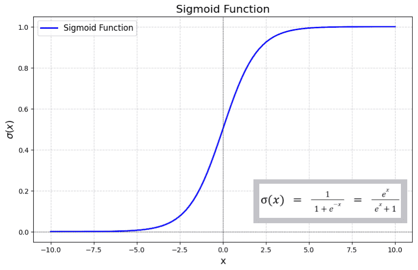
67. What is the Logistic function (Sigmoid function) in logistic regression?

The logistic function or sigmoid function, is used in logistic regression to predict probabilities. It takes any real number as input and maps it to a value between 0 and 1 which makes it great for predicting binary outcomes like "yes" or "no."

The formula looks like this:

f(x) = \frac{1}{1 + e^{-x}}

The sigmoid function helps us predict the probability of an event happening. If the output is close to 1, we predict one class and if it's close to 0, we predict the other.

Sigmoid-Activation-Function — Sigmoid Function

68. What is overfitting and how can be overcome this?

Overfitting refers to the result of analysis of a dataset which fits so closely with training data that it fails to generalize with unseen/future data. This happens when the model is trained with noisy data which causes it to learn the noisy features from the training as well.

To avoid Overfitting and overcome this problem in machine learning, one can follow the following rules:

Feature selection : Sometimes the training data has too many features which might not be necessary for our problem statement. In that case, we use only the necessary features that serve our purpose
Cross Validation : This technique is a very powerful method to overcome overfitting. In this, the training dataset is divided into a set of mini training batches which are used to tune the model.
Regularization : Regularization is the technique to supplement the loss with a penalty term so as to reduce overfitting. This penalty term regulates the overall loss function, thus creating a well trained model.
Ensemble models : These models learn the features and combine the results from different training models into a single prediction.

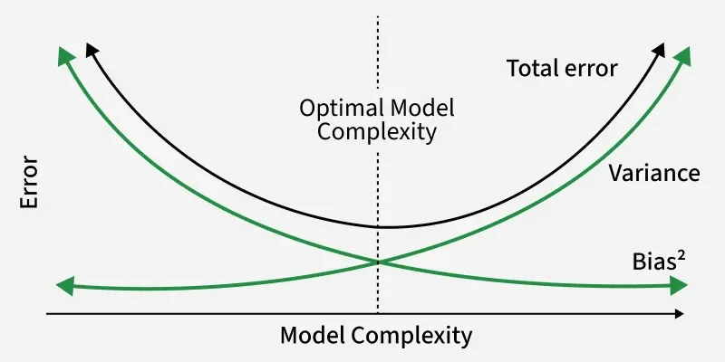
69. Explain the concepts of Bias-Variance trade-off in machine learning.

When creating predictive models, the bias-variance trade-off is a key concept in machine learning that deals with finding the right balance between two sources of error, bias and variance. It plays a crucial role in model selection and understanding the generalization performance of a machine learning algorithm. Here’s an explanation of these concepts:

Bias: It is simply described as the model’s inability to forecast the real value due of some difference or inaccuracy. These differences between actual or expected values and the predicted values are known as error or bias error or error due to bias.
Variance: It is a measure of data dispersion from its mean location. In machine learning, variance is the amount by which a predictive model’s performance differs when trained on different subsets of the training data. More specifically, variance is the model’s variability in terms of how sensitive it is to another subset of the training dataset, i.e. how much it can adapt on the new subset of the training dataset.

	Low Bias	High Bias
Low Variance	Best fit (Ideal Scenario )	Underfitting
High Variance	Overfitting	Not capture the underlying patterns (Worst Case)

70. What are the different Loss Functions used in Machine Learning?

Loss functions measure the error between predicted and actual values, guiding optimization during training:

MSE (Mean Squared Error): Regression; squares errors, penalizing larger errors more.
MAE (Mean Absolute Error): Regression; less sensitive to outliers than MSE.
Huber Loss: Combines MSE and MAE, less sensitive to outliers than pure MSE.
Cross-Entropy (Log Loss): Classification; measures difference between predicted probability and actual label.
Hinge Loss: Used in SVMs; encourages maximum margin between classes.
KL Divergence: Measures how one probability distribution differs from another.

71. What is a support vector machine (SVM) and what are its key components?

Support Vector machines are a type of Supervised algorithm which can be used for both Regression and Classification problems.

In SVMs, the main goal is to find a hyperplane which will be used to segregate different data points into classes.
Any new data point will be classified based on this defined hyperplane.
SVM finds the optimal hyperplane that separates classes while maximizing the margin between them.

The key components of SVM are:

Kernels Function: It is a mapping function used for data points to convert it into high dimensionality feature space.
Hyperplane: It is the decision boundary which is used to differentiate between the classes of data points.
Margin: It is the distance between Support Vector and Hyperplane
C: It is a regularization parameter which is used for margin maximization and misclassification minimization.

72. Explain the k-nearest neighbors (KNN) algorithm.

KNN is a "lazy learner" as it memorizes training data rather than building an explicit model, computing distances only at prediction time.

How it works:

Choose K calculate distance to all training points
Select K nearest classify by majority vote (or average for regression).
A small K risks overfitting to noise; a large K risks underfitting by over-smoothing boundaries the right K is usually found via cross-validation.

73. What is the Naïve Bayes algorithm and what are the different assumptions of Naive Bayes?

The Naïve Bayes algorithm is a probabilistic classification algorithm based on Bayes’ theorem with a “naïve” assumption of feature independence within each class. It is commonly used for both binary and multi-class classification tasks, particularly in situations where simplicity, speed and efficiency are essential.

The main assumptions that Naïve Bayes theorem makes are:

Feature independence – It assumes that the features involved in Naïve Bayes algorithm are conditionally independent, i.e., the presence/ absence of one feature does not affect any other feature
Equality – This assumes that the features are equal in terms of importance (or weight).
Normality – It assumes that the feature distribution is Normal in nature, i.e., the data is distributed equally around its mean.

74. What are Decision Trees and how do they work?

Decision trees are a popular machine learning algorithm used for both classification and regression tasks. They work by creating a tree-like structure of decisions based on input features to make predictions or decisions. Lets dive into its core concepts and how they work briefly:

Decision trees consist of nodes and edges.
The tree starts with a root node and branches into internal nodes that represent features or attributes.
These nodes contain decision rules that split the data into subsets.
Edges connect nodes and indicate the possible decisions or outcomes.
Leaf nodes represent the final predictions or decisions.

Decision-Tree

75. Explain the concepts of Entropy and Information gain in decision trees.

Entropy is like a measure of how mixed or uncertain your data is. If all the data points belong to the same class, entropy is low. If the data is spread out across many different classes, entropy is high. Formula for entropy is:

H(S) = - \sum_{i=1}^{n} p_i \log_2(p_i)

where:

p_i is the probability of each class in the dataset.

Information Gain tells us how much we reduce that uncertainty after we split the data using a feature. A higher information gain means the feature helps us organize the data better and makes it easier to predict the target class. It's the difference between the uncertainty before and after the split. Formula for information gain is:

\text{Information Gain} = H(S) - \sum_{i=1}^{k} \frac{|S_i|}{|S|} H(S_i)

where:

H(S) is the entropy before the split,
H(S_i) is the entropy of the subsets after the split,
|S_i| is the number of instances in subset, and
|S| is the total number of instances in the dataset.

76. What is Pruning in Decision Trees?

Pruning removes branches that add little predictive value, reducing overfitting and improving generalization.

Pre-Pruning (Early Stopping): Stop growth early via constraints like max depth or minimum samples per split.
Post-Pruning: Grow the full tree first, then remove branches with little impact on accuracy (e.g., Cost Complexity Pruning).

77. What is the difference between the Bagging and Boosting model?

Bagging and Boosting are two techniques used to improve the accuracy of machine learning models by combining multiple models together, but they work in different ways.

In Bagging, we train several models independently on different random parts of the data. Each model makes its own predictions and then we combine those predictions by either averaging or voting. Example: Random Forest Algorithm.
In Boosting, models are trained one after another. Each new model tries to fix the mistakes of the previous one and the final prediction is based on a combination of all models where better models are given more weight. Example: AdaBoost and Gradient Boosting.

78. Describe Random Forests and their advantages over Single-Decision Trees.

Random Forests are an ensemble learning technique that combines multiple decision trees to improve predictive accuracy and reduce overfitting. The advantages it has over single decision trees are:

Improved Generalization: Single decision trees are prone to overfitting, especially when they become deep and complex. Random Forests mitigate this issue by averaging predictions from multiple trees, resulting in a more generalized model that performs better on unseen data
Better Handling of High-Dimensional Data : Random Forests are effective at handling datasets with a large number of features. They select a random subset of features for each tree which can improve the performance when there are many irrelevant or noisy features
Robustness to Outliers: Random Forests are more robust to outliers because they combine predictions from multiple trees which can better handle extreme cases.

79. Explain the Gradient Boosting algorithms — XGBoost and CatBoost.

Gradient Boosting combines weak learners sequentially, each correcting the previous model's residual errors.

Initialize with a weak learner (e.g., a shallow tree).
Calculate the difference between target and predicted values (residuals).
Add a new weak learner to capture those residuals.
Update the model using a learning rate to control the update size.
Repeat, each iteration correcting previous errors.

XGBoost adds L1/L2 regularization and parallelization for speed and accuracy while CatBoost handles categorical features natively (no manual encoding needed) and uses ordered boosting to reduce overfitting.

80. What is K-Means and how does it work?

K-Means is an unsupervised machine learning algorithm used for clustering or grouping similar data points together. It aims to partition a dataset into K clusters where each cluster represents a group of data points that are close to each other in terms of some similarity measure. The working of K-means is as follow:

Choose the number of clusters K
For each data point in the dataset, calculate its distance to each of the K centroids and then assign each data point to the cluster whose centroid is closest to it
Recalculate the centroids of the K clusters based on the current assignment of data points.
Repeat the above steps until a group of clusters are formed.

81. What is a Confusion Matrix? Explain with an example.

Confusion matrix is a table used to evaluate the performance of a classification model by presenting a comprehensive view of the model’s predictions compared to the actual class labels. It provides valuable information for assessing the model’s accuracy, precision, recall and other performance metrics in a binary or multi-class classification problem.

A famous example demonstration would be Cancer Confusion matrix:

	Actual Cancer	Actual Not Cancer
Predicted Cancer	True Positive (TP)	False Positive (FP)
Predicted Not Cancer	False Negative (FN)	True Negative (TN)

TP (True Positive) = The number of instances correctly predicted as the positive class
TN (True Negative) = The number of instances correctly predicted as the negative class
FP (False Positive) = The number of instances incorrectly predicted as the positive class
FN (False Negative) = The number of instances incorrectly predicted as the negative class

82. What is a classification report and explain the parameters used to interpret the result of classification tasks with an example.

A classification report is a summary of the performance of a classification model, providing various metrics that help assess the quality of the model’s predictions on a classification task.

The parameters used in a classification report typically include:

Precision: Precision is the ratio of true positive predictions to the total predicted positives. It measures the accuracy of positive predictions made by the model.

Precision = TP/(TP+FP)

Recall (Sensitivity or True Positive Rate): Recall is the ratio of true positive predictions to the total actual positives. It measures the model’s ability to identify all positive instances correctly.

Recall = TP / (TP + FN)

Accuracy: Accuracy is the ratio of correctly predicted instances (both true positives and true negatives) to the total number of instances. It measures the overall correctness of the model’s predictions.

Accuracy = (TP + TN) / (TP + TN + FP + FN)

F1-Score: The F1-Score is the harmonic mean of precision and recall. It provides a balanced measure of both precision and recall and is particularly useful when dealing with imbalanced datasets.

F1-Score = 2 * (Precision * Recall) / (Precision + Recall)

83. What is Regularization in Machine Learning? State the differences between L1 and L2 regularization.

Regularization is a technique used to prevent a model from becoming too complex and overfitting the training data. It adds a penalty to the model's cost function to keep the model simpler, helping it perform better on new, unseen data.

L1 Regularization (Lasso)

It adds the absolute value of the model's coefficients to the cost function.
L1 encourages sparsity, meaning it can make some feature weights exactly zero, effectively removing those features from the model.
This is useful for feature selection.

L2 Regularization (Ridge)

It adds the square of the coefficients to the cost function.
L2 reduces the size of all coefficients but doesn’t set them to zero, keeping all features in the model but making them less influential.

84. What is Laplace smoothing (add-one smoothing) and why is it used in Naive Bayes?

If a feature value never appeared for a class in training, its probability becomes exactly zero forcing the entire posterior probability to zero regardless of other evidence.

Laplace Smoothing adds a small constant (typically 1) to every feature count, preventing zero probabilities and overconfident, incorrect predictions — especially important in text classification, where many words are unseen per class.

85. What is DBSCAN and how do we use it?

Density-Based Spatial Clustering of Applications with Noise (DBSCAN), is a density-based clustering algorithm used for grouping together data points that are close to each other in high-density regions and labeling data points in low-density regions as outliers or noise. Here is how it works:

For each data point in the dataset, DBSCAN calculates the distance between that point and all other data points
DBSCAN identifies dense regions by connecting core points that are within each other’s predefined threshold (eps) neighborhood.
DBSCAN forms clusters by grouping together data points that are density-reachable from one another.

86. How does the EM (Expectation-Maximization) algorithm work in clustering?

The Expectation-Maximization (EM) algorithm is a probabilistic approach used for clustering data when dealing with mixture models. EM is commonly used when the true cluster assignments are not known and when there is uncertainty about which cluster a data point belongs to. Here is how it works:

First, the number of clusters K to be formed is specified.
Then, for each data point, the likelihood of it belonging to each of the K clusters is calculated. This is called the Expectation (E) step
Based on the previous step, the model parameters are updated. This is called Maximization (M) step.
Together it is used to check for convergence by comparing the change in log-likelihood or the parameter values between iterations.
If it converges, then we have achieved our purpose. If not, then the E-step and M-step are repeated until we reach convergence.

87. Explain the concept of silhouette score in clustering evaluation.

Silhouette score is a metric used to evaluate the quality of clusters produced by a clustering algorithm. Here is how it works:

the average distance between the data point and all other data points in the same cluster is first calculated. Let us call this as (a)
Then for the same data point, the average distance (b) between the data point and all data points in the nearest neighboring cluster (i.e., the cluster to which it is not assigned)
silhouette coefficient for each data point is calculated which given by: S = (b – a) / max(a, b)
- if -1<S<0, it signifies that data point is closer to a neighboring cluster than to its own cluster.
- if S is close to zero, data point is on or very close to the decision boundary between two neighboring clusters.
- if 0<S<1, data point is well within its own cluster and far from neighboring clusters.

88. What is the relationship between eigenvalues and eigenvectors in PCA?

In Principal Component Analysis (PCA), eigenvalues and eigenvectors play a crucial role in the transformation of the original data into a new coordinate system. Let us first define the essential terms:

Eigen Values: Eigenvalues are associated with each eigenvector and represent the magnitude of the variance (spread or extent) of the data along the corresponding eigenvector
Eigen Vectors: Eigenvectors are the directions or axes in the original feature space along which the data varies the most or exhibits the most variance

The relationship between them is given as:

AV = \lambda{V}, where

A = Feature matrix
V = eigen vector
\lambda = Eigen value.

89. What is the Cross Validation technique in Machine Learning?

Cross-validation is a resampling technique used in machine learning to assess and validate the performance of a predictive model.

K-Fold Cross-Validation: In this, the data is divided into K subsets and K iterations of training and testing are performed.
Stratified K-Fold Cross-Validation: This technique ensures that each fold has approximately the same proportion of classes as the original dataset (helpful in handling data imbalance)
Shuffle-Split Cross-Validation: It randomly shuffles the data and splits it into training and testing sets.

90. What are the ROC and AUC? Explain their significance in binary classification.

Receiver Operating Characteristic (ROC) is a graphical representation of a binary classifier’s performance. It plots the true positive rate (TPR) vs the false positive rate (FPR) at different classification thresholds.

True positive rate (TPR) : It is the ratio of true positive predictions to the total actual positives.

Recall = TP / (TP + FN)

False positive rate (FPR) : It is the ratio of False positive predictions to the total actual positives.

FPR= FP / (TP + FN)

91. What is Hyperparameter Tuning, and what are the common methods?

Finding the best hyperparameter combination (learning rate, tree depth, etc.) to maximize performance:

Grid Search: Exhaustively tries every combination — thorough but expensive.
Random Search: Randomly samples combinations — often faster, good results in fewer iterations.
Bayesian Optimization: Builds a probabilistic model to intelligently choose the next combination to try — efficient for expensive models.

92. Describe Batch Gradient Descent, Stochastic Gradient Descent and Mini-Batch Gradient Descent.

1. Batch Gradient Descent

In Batch Gradient Descent, the entire training dataset is used to compute the gradient of the cost function with respect to the model parameters (weights and biases) in each iteration.
This means that all training examples are processed before a single parameter update is made.
It converges to a more accurate minimum of the cost function but can be slow, especially in a high dimensionality space.

2. Stochastic Gradient Descent

In Stochastic Gradient Descent, only one randomly selected training example is used to compute the gradient and update the parameters in each iteration.
The selection of examples is done independently for each iteration.
This is capable of faster updates and can handle large datasets because it processes one example at a time but high variance can cause it to converge slower.

3. Mini-Batch Gradient Descent

Mini-Batch Gradient Descent strikes a balance between BGD and SGD.
It divides the training dataset into small, equally-sized subsets called mini-batches.
In each iteration, a mini-batch is randomly sampled and the gradient is computed based on this mini-batch.
It utilizes parallelism well and takes advantage of modern hardware like GPUs but can still exhibits some level of variance in updates compared to Batch Gradient Descent.

93. How can you prevent Gradient Descent from getting stuck in local minima?

Local minima happen when the algorithm gets stuck in a small minimum point, instead of finding the best solution. To avoid this:

Good Starting Point: Use techniques like Xavier/Glorot or He initialization to set good starting values for the model’s weights.
Smart Optimizers: Use optimizers like Adam or RMSProp that adjust the learning speed based on past steps, helping the algorithm move past local minima.
Randomness with Mini-Batches: Use mini-batch gradient descent which introduces some randomness allowing the algorithm to jump out of local minima.
Increase Model Complexity: Adding more layers or neurons can create a more complex model, reducing the chance of getting stuck.
Tune Hyperparameters: Try different settings for the model using methods like random search or grid search to find the best ones.

94. What is Artificial Neural Networks?

Artificial Neural Networks take inspiration from structure and functioning of human brain. The computational units in ANN are called neurons and these neurons are responsible to process and pass the information to the next layer.

ANN has three main components:

Input Layer: where the network receives input features.
Hidden Layer: one or more layers of interconnected neurons responsible for learning patterns in the data
Output Layer: provides final output on processed information.

95. What are Activation Functions, and why are they needed?

An activation function introduces non-linearity, letting the network learn complex patterns instead of collapsing into a single linear transformation.

Sigmoid: Squashes output to (0,1); used for binary outputs, but prone to vanishing gradients.
Tanh: Squashes to (-1,1); zero-centered, still vanishing-gradient prone.
ReLU:max(0, x); most widely used in hidden layers — efficient and mostly avoids vanishing gradients, though can suffer "dying ReLU."
Softmax: Converts outputs into a probability distribution — used in multi-class output layers.

96. What is the forward and backward propogations in deep learning?

Forward Propagation: Input data passes through the network layer by layer, with each neuron applying weights, biases, and an activation function, until the output layer produces a prediction.
Backward Propagation: The error between the prediction and actual value is propagated backward using the chain rule, computing gradients for each weight and bias — these gradients are then used to update the parameters and reduce future error.

97. What is the Vanishing and Exploding Gradient Problem?

Vanishing Gradients: Gradients shrink exponentially through many layers, causing early layers to learn very slowly — common with Sigmoid/Tanh in deep/recurrent networks.
Exploding Gradients: Gradients grow exponentially instead, causing unstable updates.

Solutions: ReLU activation, gradient clipping, proper weight initialization (Xavier/He), and architectures like LSTM/GRU designed specifically to combat this in sequential data.

98. Explain the convolution operations of CNN architecture.

In a Convolutional Neural Network (CNN), convolutions help the model find important features in images like edges or textures.

Small filters (also called kernels) slide over the image, checking one small part at a time.
These filters look for patterns by doing a calculation at each position, creating something called a feature map.
The strides control how far the filter moves at each step.
This helps the network recognize the same feature, even if it's in a different part of the image.
After convolutions, pooling layers shrink the feature maps, keeping the important details while making the data smaller and faster to process.

99. What is Feed Forward Network and how it is different from Recurrent Neural Network?

Deep learning designs that are basic are feedforward neural networks and recurrent neural networks. They are both employed for different tasks, but their structure and how they handle sequential data differ.

Feed Forward Neural Network

In FFNN, the information flows in one direction, from input to output, with no loops
It consists of multiple layers of neurons, typically organized into an input layer, one or more hidden layers and an output layer.
Each neuron in a layer is connected to every neuron in the subsequent layer through weighted connections.
FNNs are primarily used for tasks such as classification and regression where they take a fixed-size input and produce a corresponding output

Recurrent Neural Network

A recurrent neural network is designed to handle sequential data where the order of input elements matters. Unlike FNNs, RNNs have connections that loop back on themselves allowing them to maintain a hidden state that carries information from previous time steps.
This hidden state enables RNNs to capture temporal dependencies and context in sequential data, making them well-suited for tasks like natural language processing, time series analysis and sequence generation.
However, standard RNNs have limitations in capturing long-range dependencies due to the vanishing gradient problem.

100. What is the differnce between RNN , LSTM , GRU?

RNN (Recurrent Neural Network), LSTM (Long Short-Term Memory), and GRU (Gated Recurrent Unit) are neural network architectures designed for processing sequential data.

RNN (Recurrent Neural Network)

RNN is a neural network designed to process sequential data by using information from previous time steps.
It maintains a hidden state that captures information from earlier inputs in the sequence.
It struggles with the vanishing gradient problem, making it difficult to learn long-term dependencies.
It has a simpler architecture with fewer parameters than LSTM and GRU.
It is suitable for short sequences where long-term memory is not required.
Goal: Learn patterns and dependencies in sequential data.

LSTM (Long Short-Term Memory)

LSTM is an advanced type of RNN designed to overcome the vanishing gradient problem.
It uses a memory cell along with input, forget, and output gates to control the flow of information.
It can retain information over long sequences, making it effective for long-term dependencies.
It has a more complex architecture and requires more computational resources.
It is widely used in language modeling, speech recognition, and time-series forecasting.
Goal: Capture long-term dependencies in sequential data.

GRU (Gated Recurrent Unit)

GRU is a simplified version of LSTM that also addresses the vanishing gradient problem.
It uses only update and reset gates instead of three gates.
It does not have a separate memory cell; the hidden state stores the required information.
It has fewer parameters than LSTM, making it faster to train.
It often achieves performance comparable to LSTM while requiring less computation.
Goal: Efficiently capture sequence dependencies with a simpler architecture.

101. How does LSTM resolve the Vanishing Gradient Problem of RNN?

Standard RNNs suffer from vanishing gradients because the same weight matrix is repeatedly multiplied at every time step during backpropagation, causing gradients to shrink exponentially over long sequences.

LSTM solves this using a separate cell state that runs through the entire sequence with only minor linear modifications (addition/multiplication by gate values), rather than repeated full weight-matrix multiplication.
The Forget Gate controls what to discard, the Input Gate controls what new information to add, and this additive update mechanism allows gradients to flow backward through many time steps largely unchanged preventing them from vanishing the way they do in a standard RNN.

102. Explain the difference between generative and discriminative models?

Generative models and discriminative models are used for different purposes in machine learning.

Generative models try to understand how data is generated, meaning they learn the relationship between input data 𝑋 and target labels 𝑌. This allows them to create new data that looks like the original dataset.
On the other hand, discriminative models focus on distinguishing between different classes or making predictions based on the input data. They learn the relationship between the input 𝑋 and the target 𝑌 directly, without trying to generate new data.

103. Explain the concept of Word Embeddings in NLP.

Word Embeddings represent words as dense vectors capturing semantic meaning — similar words get similar vectors, based on the idea that words in similar contexts have similar meanings. Common techniques: Word2Vec, GloVe, TF-IDF, and contextual embeddings from BERT.

104. What is a Seq2Seq Model?

A Sequence-to-Sequence (Seq2Seq) model handles tasks involving variable-length input and output sequences widely used in machine translation, text summarization, and question answering.

An Encoder processes the input sequence into a fixed-length context vector capturing its meaning.
A Decoder then takes that vector and generates the output sequence step-by-step, often using each predicted output as input for generating the next one (autoregressive generation).

105. What is the Attention Mechanism, and how do Transformers use it?

The Attention Mechanism allows a model to focus on the most relevant parts of the input sequence when producing each part of the output, rather than compressing the entire input into a single fixed-length vector (a major limitation of basic Seq2Seq models).

Transformers are built entirely around self-attention every word in a sequence can directly attend to every other word, weighted by relevance, capturing both short and long-range dependencies.
Unlike RNNs, Transformers process the entire sequence in parallel rather than step-by-step, making them significantly faster to train and better at capturing long-range context the architecture behind models like BERT and GPT.

106. What is Transfer Learning, and how is it applied in Deep Learning?

Reuses a model already trained on one task to help solve a related task, instead of training from scratch.
Feature Extraction (use pretrained features, drop final layers) followed by Fine-Tuning (adjust weights on the new, often smaller, target dataset)
It saves time and often outperforms training from scratch, especially with limited labeled data.

107. What is Generative AI?

Generative AI is an abbreviation for Generative Artificial Intelligence which refers to a class of artificial intelligence systems and algorithms that are designed to generate new, unique data or material that is comparable to or indistinguishable from, human-created data. It is a subset of artificial intelligence that focuses on the creative component of AI allowing machines to develop innovative outputs such as writing, graphics, audio and more.

Generative AI models such as GPT (Generative Pretrained Transformer) can generate human-like text.” Natural language synthesis, automated content production and chatbot responses are all common uses for these models.
Images are generated using generative adversarial networks (GANs).” GANs are made up of a generator network that generates images and a discriminator network that determines the authenticity of the generated images. Because of the struggle between the generator and discriminator, high-quality, realistic images are produced.
Generative AI can also create audio content such as speech synthesis and music composition.” Audio content is generated using models such as WaveGAN and Magenta.

108. What is the difference between GANs and VAEs?

Both are generative deep learning architectures, but they work very differently:

GAN (Generative Adversarial Network): Consists of two competing networks a Generator that creates fake data and a Discriminator that tries to distinguish fake from real data. The two are trained together in an adversarial process, pushing the Generator to produce increasingly realistic outputs. GANs typically produce sharper, more photorealistic images.
VAE (Variational Autoencoder): Learns a probabilistic mapping from data into a compressed latent space using an Encoder, then reconstructs data from that space using a Decoder. VAEs produce smoother, more controllable outputs but are generally blurrier than GANs, since they optimize for a probabilistic reconstruction rather than adversarial realism.

When to use which: GANs for high-fidelity image generation; VAEs when you need a structured, interpretable latent space (e.g., for controlled data generation or interpolation).

109. What are Large Language Models (LLMs) and what does "fine-tuning" mean?

LLMs (like GPT, BERT-based models) are large Transformer-based models pretrained on massive amounts of text to learn general language patterns, grammar, and world knowledge.
Fine-tuning takes this pretrained model and further trains it on a smaller, task-specific dataset — adapting its general knowledge to a specialized use case (e.g., fine-tuning GPT on customer support transcripts to build a domain-specific chatbot) — without needing to train a model from scratch, which would require far more data and compute.

Data Science Interview Questions and Answers

1. What is the difference between Data Science and Data Analytics?

2. What are the different types of data used in Data Science?

3. What is the Data Science Lifecycle?

4. What is the difference between Data Science, Machine Learning, and Artificial Intelligence?

5. What is the difference between Data Science and Data Engineering?

6. What is Python and why is it widely used in Data Science?

7. What is the difference between a List and a Tuple in Python?

8. What is NumPy and why is it faster than regular Python lists?

9. What is Pandas and what are its main data structures?

10. How do you handle missing values in Pandas?

11. What is SQL, and what does it stand for?

12. What is the difference between SQL and NoSQL databases?

13. What are the main components (clauses) of a SQL query and in what order do they execute?

14. What is the difference between a Primary Key and a Foreign Key?

15. What is the difference between the WHERE and HAVING clause?

16. What is the difference between INNER JOIN, LEFT JOIN, RIGHT JOIN, and FULL JOIN?

17. What are Window Functions and how do they differ from Aggregate Functions?

18. What's the difference between COUNT(*), COUNT(1), and COUNT(column_name) ?

19. What is the difference between a JOIN and a SUBQUERY, and when would you use each?

20. What is a CTE (Common Table Expression) and how is it different from a Subquery?

21. What are Indexes in SQL and how do they improve performance?

22. What are ACID properties in DBMS?

23. What is the difference between Normalization and Denormalization?

24. What are Views and Stored Procedures in SQL?

25. What is Data Visualization and why is it important in Data Science?

26. What are the commonly used Data Visualization libraries/tools in Python?

27. When would you use a Bar Chart, Histogram, Box Plot, or Scatter Plot?

28. How would you visually detect skewness in a dataset?

29. What is a Random Variable? Explain Discrete vs Continuous Random Variables.

30. What is Marginal Probability?

31. What are the Probability Axioms?

32. What is the difference between Dependent and Independent Events in Probability?

33. What is Conditional Probability?

34. What is Bayes’ Theorem and when do we use it in Data Science?

35. Define Variance and Conditional Variance.

36. Explain the concepts of Mean, Median, Mode and Standard Deviation.

37. What are Skewness and Kurtosis?

38. What is Normal Distribution and Standard Normal Distribution?

39. What is the Empirical Rule (68-95-99.7 Rule)?

40. What is the difference between correlation and causation?

41. What are Uniform, Bernoulli and Binomial Distributions and how do they differ?

42. Describe the Poisson Distribution and its characteristics.

43. Explain the t-distribution and its relationship with the normal distribution.

44. Describe the chi-squared distribution.

45. What is the difference between z-test, F-test and t-test?

46. What is the central limit theorem and why is it significant in statistics?

47. Describe the process of hypothesis testing, including null and alternative hypotheses.

48. How do you calculate a confidence interval and what does it represent?

49. What is a p-value in statistics?

50. Explain Type I and Type II errors in hypothesis testing.

51. What is the significance level (alpha) in hypothesis testing?

52. How can you calculate the correlation coefficient between two variables?

53. What is covariance and how is it related to correlation?

54. Explain how to perform a hypothesis test for comparing two population means.

55. What is ANOVA? What are the different ways to perform ANOVA tests?

56. What is Exploratory Data Analysis (EDA) and why is it important?

57. What are the key steps involved in Data Preprocessing?

58. What are outliers, and how do you detect and handle them?

59. What is Feature Engineering, and why does it matter?

60. What is the difference between Label Encoding and One-Hot Encoding?

61. What is Upsampling and Downsampling?

62. What is the Curse of Dimensionality?

63. Explain PCA (Principal Component Analysis) and how it works.

64. What are the different types of machine learning?

65. What is linear regression and what are the different assumptions of linear regression algorithms?

66. Logistic Regression is a classification technique and why is its name regression not Logistic Classification?

67. What is the Logistic function (Sigmoid function) in logistic regression?

68. What is overfitting and how can be overcome this?

69. Explain the concepts of Bias-Variance trade-off in machine learning.

70. What are the different Loss Functions used in Machine Learning?

71. What is a support vector machine (SVM) and what are its key components?

72. Explain the k-nearest neighbors (KNN) algorithm.

73. What is the Naïve Bayes algorithm and what are the different assumptions of Naive Bayes?

74. What are Decision Trees and how do they work?

75. Explain the concepts of Entropy and Information gain in decision trees.

76. What is Pruning in Decision Trees?

77. What is the difference between the Bagging and Boosting model?

78. Describe Random Forests and their advantages over Single-Decision Trees.

79. Explain the Gradient Boosting algorithms — XGBoost and CatBoost.

18. What's the difference between `COUNT(*)`, `COUNT(1)`, and `COUNT(column_name)` ?