The Agent that Doesn’t Know Itself

20 March, 2026

guest post by William Waites

The previous post introduced the plumbing calculus: typed channels, structural morphisms, two forms of composition, and agents as stateful morphisms with a protocol for managing their state. The examples were simple. This post is about what happens when the algebra handles something genuinely complex.

To get there, we need to understand a little about how large language models work. These models are sequence-to-sequence transducers: a sequence of tokens comes in, a sequence comes out. Text is tokenised and the model operates on the tokens.

From the outside, the morphism is simple: !string → !string. A message goes in, a message comes out. But the client libraries (the code that calls the LLM provider) maintain the conversation history and send it back with every call. The actual morphism is
(!string, ![Message]) → (!string, ![Message]): the input message and the accumulated history go in, the response and the updated history come out. The history feeds back. This is a trace in the sense of traced monoidal categories: the feedback channel is hidden from the user, who sees only !string → !string.

Crucially, the model has a limited amount of memory. It is not a memoryless process, but the memory it has is not large: 200,000 tokens for current models, perhaps a million for the state of the art. This sounds like a lot. It is not. An academic paper is roughly 10,000 tokens. A literature review that needs to work with thirty papers has already exceeded the context window of most models, and that is before the model has produced a single word of output.

If you have used any of these agent interfaces, you will have noticed that after talking back and forth for a while, the agent will compact. This is a form of memory management. What is happening is that some supervisory process has noticed the context window filling up, and has intervened to shorten its contents. A naïve approach is to truncate: discard everything before the last N exchanges. A better approach is to feed the entire context to another language model and ask it to summarise, then put the summary back.

This is normally done by specialised code outside the agent, invisible to it.

How to manage agent memory well is an active research area. We do not, in general, do it very well. Truncation loses information. Summarisation loses nuance. Pinning helps but the right pinning strategy depends on the task. These are open questions, and to make progress we need to be able to experiment with different schemes and mechanisms: express a memory management strategy, test it, swap it for another, compare. Not by recompiling specialised code or hardcoding behaviour, but by writing it down in a language designed for exactly this kind of composition. Memory management should be a plumbing program: modular, type-checked, swappable.

So we built an implementation of compaction using the plumbing calculus, and the first thing we did was test it. I ran the protocol on a very short cycle: a single message caused a compaction, because the threshold was set to zero for testing. The compressor fired, produced a summary, rebuilt the agent’s context. The logs showed [compressor] 3404 in / 541 out. The protocol worked.

Then I asked the agent: "have you experienced compaction?"

The agent said no. It explained what compaction is, accurately. Said it hadn’t happened yet. It was confident.

I asked: "do you have a context summary in your window?"

Yes, it said, and described the contents accurately.

"How did that context summary get there if you have not yet compacted?"

The agent constructed a plausible, confident, and completely wrong explanation: the summary was "provided to me by the system at the start of this conversation" as a "briefing or recap." When pressed, it doubled down:

"The context-summary is not evidence that compaction has occurred. It’s more like a briefing or recap that the system gives me at the start of a conversation session to provide continuity."

The agent was looking at the direct evidence of its own compaction and confidently explaining why it was not compaction. We will return to why it gets this wrong, and how to fix it. But first: how do we build this?

The compacting homunculus

At a high level, it works like this. An agent is running: input comes in, output goes out. Together with the output, the agent emits a telemetry report. The telemetry includes token counts: with each transaction, the entire train of messages and responses is sent to the LLM provider, and back comes a response together with a count of the tokens that went in and the tokens that came out. Our agent implementation sends this telemetry out of the telemetry port to anybody who is listening.

The construction involves a second agent. This second agent is a homunculus: the little man who sits on your shoulder and watches what your mind is doing. Here is the topology:

Topology of the compacting homunculus. Two boxes: Agent (large, bottom) and Compressor (smaller, top). The Agent has input and output ports for the main data flow (dark blue arrows). Three channels connect the Agent to the Compressor: telemetry flows up from the Agent (the Compressor watches token counts), ctrl_out flows up from the Agent (the Compressor receives acknowledgements), and ctrl_in flows down from the Compressor to the Agent (the Compressor sends commands). The Agent does not know the Compressor exists. It just receives control messages and responds to them.

The homunculus listens to the telemetry and says: the memory is filling up. The token count has crossed a threshold. It is time to compact. And then it acts:

• Send pause to the agent’s control port. Stop accepting input.
• Send get memory. The agent produces the contents of its context window.
• Summarise that memory (using another LLM call).
• Send set memory with the compacted version.
• Send resume. The agent continues processing input.

Each step requires an acknowledgement before the next can proceed. This is a protocol: pause, acknowledge, get memory, here is the memory, set memory, acknowledge, resume, acknowledge.

It is possible to express this directly in the plumbing calculus, but it would be painfully verbose. Instead, we use session types to describe the protocol. This is not pseudocode. There is a compiler and a runtime for this language. Here is the protocol:

protocol Compaction =
  send Pause . recv PauseAck .
  send GetMemory . recv MemoryDump .
  send SetMemory . recv SetMemoryAck .
  send Resume . recv ResumeAck . end

The protocol is eight lines. It reads as a sequence of steps:
send, receive, send, receive, and so on. The compiler knows what
types each step carries. Now we wire it up:

let compact : (!CtrlResp, !json) -> !CtrlCmd =
  plumb(ctrl_out, telemetry, ctrl_in) {

    (ctrl_out, ctrl_in)  Compaction as session

    telemetry
      ; filter(kind = "usage" && input_tokens > 150000)
      ; map(null) ; session@trigger

    session@trigger ; map({pause: true})
      ; session@send(Pause)
    session@done(PauseAck) ; map({get_memory: true})
      ; session@send(GetMemory)
    session@recv(MemoryDump) ; compressor
      ; session@send(SetMemory)
    session@done(SetMemoryAck) ; map({resume: true})
      ; session@send(Resume)
}

The first line binds the protocol to the agent’s control ports:

(ctrl_out, ctrl_in) <-> Compaction as session.

This says: the Compaction protocol runs over the control channel, and we refer to it as session. The telemetry line is the trigger: when token usage crosses a threshold, the protocol begins. Each subsequent line is one step of the protocol, wired to the appropriate control
messages.

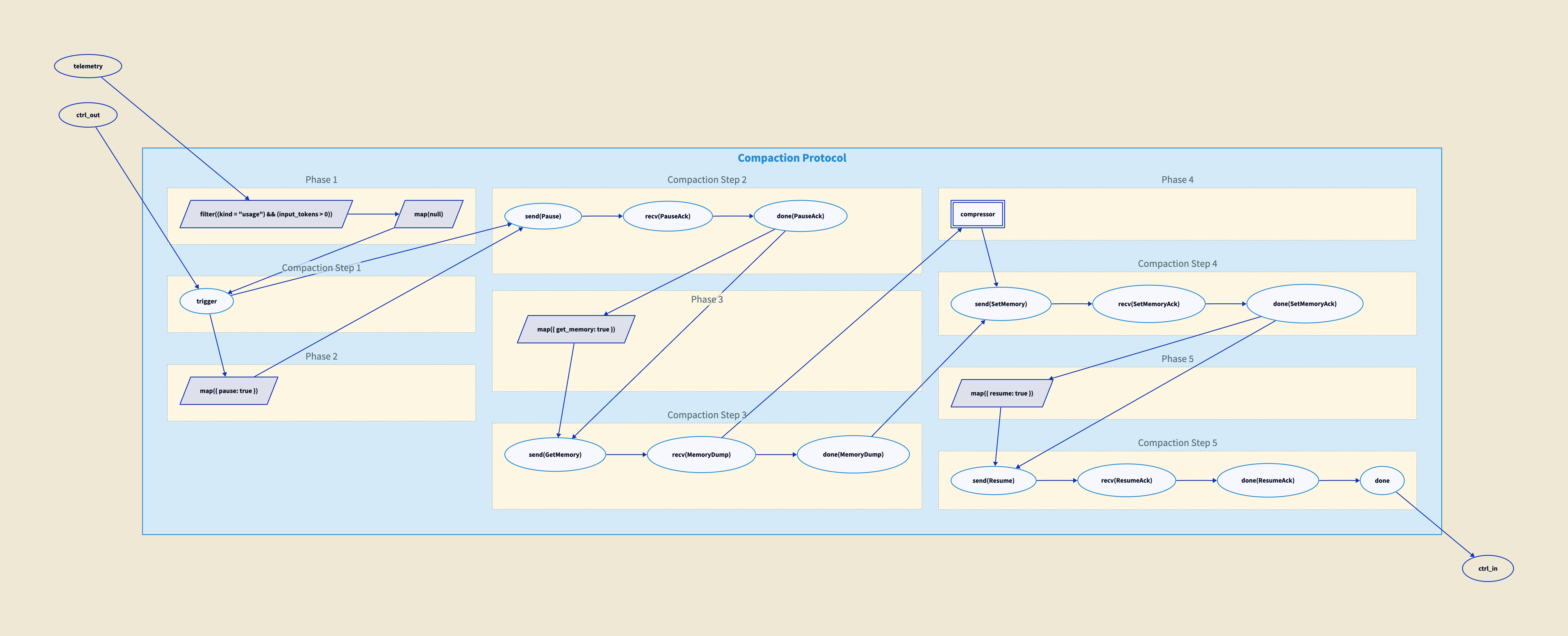
Here is a direct depiction of the protocol as wired. You can trace it through:

Diagram of the compaction protocol wired between the homunculus and the bot agent. Shows the telemetry stream flowing from the bot to the homunculus, a filter checking token usage against a threshold, and then a sequence of control messages: Pause flows to ctrl_in, PauseAck returns on ctrl_out, GetMemory flows in, MemoryDump returns, passes through a compressor agent, SetMemory flows in, SetMemoryAck returns, Resume flows in, ResumeAck returns. The protocol steps are connected in sequence. This is a direct transcription of the session type protocol into a wiring diagram.

And here is how we wire the homunculus to the agent:

let main : !string -> !string =
  plumb(input, output) {
    let ctrl : !CtrlCmd = channel
    let ctrl_out : !CtrlResp = channel
    let telem : !json = channel

    spawn bot(input=input, ctrl_in=ctrl,
              output=output, ctrl_out=ctrl_out,
              telemetry=telem)
    spawn compact(ctrl_out=ctrl_out,
                  telemetry=telem, ctrl_in=ctrl)
}

The main morphism takes a string input and produces a string output. Internally, it creates three channels (control commands, control responses, telemetry) and spawns two processes: the bot agent and the compact homunculus. The homunculus listens to the bot’s telemetry and control responses, and sends commands to the bot’s control input. The bot does not know the homunculus exists. It just receives control messages and responds to them.

There are two nested traces here. The first is the one from before, inside the agent: messages go in, the output accumulates with everything that came before, and the whole history feeds back on the next turn. We do not see this trace. It is hidden inside the client library. The second trace is the one we have just built: the homunculus. What goes around the outer loop is control: telemetry flows out, commands flow in, acknowledgements come back. The memory dump passes through the control channel at one point in the protocol, but the feedback path is control, not conversation history. Nested traces compose; the algebra has identities for this and it is fine. But they are different loops carrying different things.

Session types as barrier chains

The connection between the protocol above and what the compiler actually produces is the functor from session types into the plumbing calculus. This functor works because of barrier.

Why do we need the barrier? Because the protocol is about sending a message and waiting for a response. We can send a message, but we need the response to arrive before we proceed. The barrier takes two streams, one carrying the "done" signal and one carrying the response, and synchronises them into a pair. Only when both are present does the next step begin.

Each session type primitive has a direct image in the plumbing category, and the structure is prettier than it first appears. The primitives come in dual pairs:

In the diagrams below, session types are on the left in blue; their images in the plumbing calculus are on the right in beige.

send and recv are dual. They map to map and filter, which are also dual: send wraps the value with map, then synchronises via barrier with the done signal from the previous step. Recv filters the control output by step number, synchronises via barrier, then extracts the payload with map.

select and offer are dual. They map to tag and case analysis, which are also dual: select tags the value with a label via map, synchronises via barrier, and routes to the chosen branch chain. Offer copies the control output and filters each copy by label, routing to the appropriate branch chain.

Diagram showing the two dual pairs of session type primitives and their images in the plumbing calculus. Session types are shown in blue on the left; plumbing calculus images in beige on the right. Top section: send T is a simple arrow carrying type T; its image is map(wrap) followed by barrier with a done signal, then routing to the control input. recv T is its dual: filtering ctrl_out by step number, barrier with done, then map to extract the payload. Bottom section: select with labelled alternatives maps to coproduct injection via map(tag), barrier, then routing to the chosen branch chain. offer is its dual: copy the control output, filter each copy by label, and route to the corresponding branch chain.

• The sequencing operator (.) maps to a barrier chain. Each send-then-recv step becomes a barrier that synchronises the outgoing message with the incoming acknowledgement, and these barriers chain together to enforce the protocol ordering.

Diagram showing how the sequencing operator in session types maps to a barrier chain in the plumbing calculus. Top: the session type sequence "send T1 . recv T2 . send T3" shown as three boxes in a row connected by dots. Bottom: the plumbing image, a chain of barriers. Each send-recv pair becomes a barrier that takes the outgoing message on one arm and the incoming acknowledgement on the other, producing a synchronised pair. The done signal from one barrier feeds into the next, creating a chain that enforces protocol ordering. The trigger input starts the chain; the done output signals completion. Filters select responses by step number; maps construct outgoing messages.

rec maps to a feedback loop: merge takes the initial
arm signal and the last done signal from the previous iteration, feeds them into the barrier chain body, and copy at the end splits done into output and feedback. The trigger serialisation gate starts

end is implicit: the chain simply stops. Discard handles any remaining signals.

Diagram showing three more session type primitives and their plumbing images. Top: rec X . S (recursion) maps to a feedback loop. A merge node takes two inputs: the initial arm signal and the last-done signal fed back from the end of the body. The body is a barrier chain (S). At the output, copy splits the done signal into an output arm and a feedback arm that loops back to merge. Middle: end is shown as simply discarding any remaining signal. Bottom: the trigger and serialisation gate, which starts the protocol. A trigger input feeds through a barrier that synchronises with a copy of the done signal, ensuring only one instance of the protocol runs at a time.

This mapping is a functor. It is total: every session type primitive has an image in the plumbing category, using only the morphisms we already have. Session types are a specification language; the plumbing calculus is the execution language. The compiler translates one into the other.

The reason we do this becomes obvious from the diagram below. It is scrunched up and difficult to look at. If you click on it you can get a big version and puzzle it out. If you squint through the spaghetti, you can see that it does implement the same compaction protocol above. We would not want to implement this by hand. So it is nice to have a functor. If you have the patience to puzzle your way through it, you can at least informally satisfy yourself that it is correct.

Thumbnail of the fully desugared compaction protocol as produced by the compiler. The diagram is intentionally dense: a large network of barriers, filters, maps, copy and merge nodes, all connected by typed wires. Each step of the compaction protocol (pause, get memory, set memory, resume) is visible as a cluster of barrier chains with filters selecting response types and maps constructing commands. The full-size version is linked for readers who want to trace the individual connections, but the point is that this is what the compiler produces from the eight-line session type specification above, and you would not want to construct it by hand.

Document pinning

There is another feature we implement, because managing the memory of an agent is not as simple as just compressing it.

The problem with compression is that it is a kind of annealing. As the conversation grows, it explores the space of possible conversation. When it gets compacted, it is compressed, and that lowers the temperature. Then it grows again, the temperature rises, and then it is compressed again. With each compression, information is lost. Over several cycles of this, the agent can very quickly lose track of where it was, what you said at the beginning, what it was doing.

We can begin to solve this with document pinning. The mechanism is a communication between the agent and its homunculus, not shown in the protocol above. It is another protocol. The agent says: this document that I have in memory (technically a tool call and response, or just a document in the case of the prompts), pin it. What does that mean? When we do compaction, we compact the contents of memory, but when we replace the memory, we also replace those pinned documents verbatim. And of course you can unpin a document and say: I do not want this one any more.

Either the agent can articulate this or the user can. The user can say: you must remember this, keep track of this bit of information. And the agent has a way to keep the most important information verbatim, without it getting compacted away.

This accomplishes two things.

First, it tends to keep the agent on track, because the agent no longer loses the important information across compaction cycles. The annealing still happens to the bulk of the conversation, but the pinned documents survive intact.

Second, it has to do with the actual operation of the underlying LLM on the GPUs. When you send a sequence of messages, this goes into the GPU and each token causes the GPU state to update. This is an expensive operation, very expensive. This is why these things cost so much. What you can do with some providers is put a cache point and say: this initial sequence of messages, from the beginning of the conversation up until the cache point, keep a hold of that. Do not recompute it. When you see this exact same prefix, this exact same sequence of messages again, just load that memory into the GPU directly. Not only is this a lot more efficient, it is also a lot cheaper, a factor of ten cheaper if you can actually hit the cache.

So if you are having a session with an agent and the agent has to keep some important documents in its memory, it is a good idea to pin them to the beginning of memory. You sacrifice a little bit of the context window in exchange for making sure that, number one, the information in those documents is not forgotten, and number two, that it can hit the cache. This is explained in more detail in a separate post on structural prompt preservation.

The agent that doesn’t know itself

Why does the agent get this wrong? In one sense, it is right. It has not experienced compaction. Nobody experiences compaction. Compaction happens in the gap between turns, in a moment the agent cannot perceive. The agent’s subjective time begins at the summary. There is no "before" from its perspective.

The summary is simply where memory starts. It is like asking someone "did you experience being asleep?" You can see the evidence, you are in bed, time has passed. But you did not experience the transition.

The <context-summary> tag is a structural marker. But interpreting it as evidence of compaction requires knowing what the world looked like before, and the agent does not have that. It would need a memory of not having a summary, followed by a memory of having one. Compaction erases exactly that transition.

Self-knowledge as metadata

The fix is not complicated. It is perfectly reasonable to provide, along with the user’s message, self-knowledge to the agent as metadata. What would it be useful for the agent to know?

The current time. The sense of time that these agents have is bizarre. We live in continuous time. Agents live in discrete time. As far as they are concerned, no time passes between one message and the next. It is instantaneous from their point of view. You may be having a conversation, walk away, go to the café, come back two hours later, send another message, and as far as the agent is concerned no time has passed. But if along with your message you send the current time, the agent knows.

How full the context window is. The agent has no way of telling, but you can provide it: this many tokens came in, this many went out.

Compaction cycles. So the agent knows how many times it has been compacted, and can judge the accuracy of the contents of its memory, which otherwise it could not do.

With the compaction counter, the agent immediately gets it right:

"Yes, I have experienced compaction. According to the runtime context, there has been 1 compaction cycle during this session."

No hedging, no confabulation. Same model, same prompts, one additional line of runtime context.

Context drift

This matters beyond the compaction story, because many of the failures we see in the news are context failures, not alignment failures.

While we were writing this post, a story appeared in the Guardian about AI chatbots directing people with gambling addictions to online casinos. This kind of story is common: vulnerable people talking to chatbots, chatbots giving them bad advice. The response of the industry is always the same: we need better guardrails, better alignment, as though the chatbots are badly aligned.

I do not think that is what is happening. What is happening is a lack of context. Either the chatbot was never told the person was vulnerable, or it was told and the information got lost. Someone with a gambling addiction may start by saying "I have a gambling problem." Then there is a four-hour conversation about sports. Through compaction cycles, what gets kept is the four hours of sports talk. The important bit of information does not get pinned and does not get kept. Context drift. By the time the user asks for betting tips, the chatbot no longer knows it should not give them.

The way to deal with this is not to tell the language model to be more considerate. The way to deal with it is to make sure the agent has enough information to give good advice, and that the information does not get lost. This is what document pinning is for: pinned context survives compaction, stays at the top of the window, cannot be diluted by subsequent conversation. This is discussed further in a separate post on structural prompt preservation.

But pinning is only one strategy. The field is in its infancy. We do not really know the right way to manage agent memory, and we do not have a huge amount of experience with it. What we are going to need is the ability to experiment with strategies: what if compaction works like this? What if pinning works like that? What if the homunculus watches for different signals? Each of these hypotheses needs to be described clearly, tested, and compared. This is where the formal language earns its keep. A strategy described in the plumbing calculus is precise, checkable, and can be swapped out for another without rewriting the surrounding infrastructure. We can experiment with memory architectures the way we experiment with any other part of a system: by describing what we want and seeing if it works.

Why has nobody done this?

When the first draft of this post was written, it was a mystery why the field had not thought to give agents self-knowledge as a routine matter: what they are doing, who they are talking to, what they should remember. Prompts are initial conditions. They get compacted away. There are agents that save files to disc, in a somewhat ad hoc way, but we do not give them tools to keep track of important information in a principled way.

Contemporaneously with this work, some providers have started to do it. For example, giving agents a clock, the ability to know what time it is. This is happening now, in the weeks between drafting and publication. The field is only now realising that agents need a certain amount of self-knowledge in order to function well. The compressed timeline is itself interesting: the gap between "why has nobody done this?" and "everybody is starting to do this" was a matter of weeks.

The mechanisms we have presented here allow us to construct agent networks and establish protocols that describe rigorously how they are meant to work. We can describe strategies for memory management in a formal language, test them, and swap them out. And perhaps beyond the cost savings and the efficiency increases, the ability to experiment clearly and formally with how agents manage their own memory is where the real value lies.


Formal Scientific Modeling

21 December, 2025

In January I’m going to a workshop on category theory for modeling, with a focus on epidemiology.

Formal scientific modeling: a case study in global health, 2026 January 12-16, American Institute of Mathematics, Pasadena, California. Organized by Nina Fefferman, Tim Hosgood, and Mary Lou Zeeman.

It’s sponsored by American Institute of Mathematics, the NSF, the Topos Institute, and the US NSF Center for Analysis and Prediction of Pandemic Expansion. Here are some of the goals:

1. Get a written problem list from a bunch of modelling experts, i.e. statements of the form “I’ll be interested in categorical approaches to modelling when they can do X”, or “how would category theory think about this specific dynamical behaviour, or is this actually not a category theory question at all?”, or … and so on.

2. Make academic friends. There will be people who are not at all category theorists (many of them haven’t even heard of the subject) but who have elected to spend 5 days at a working conference to actually work with some category theorists.

3. There will probably be a lot of conversations that are essentially 5–15 minute speed tutorials in “what is agro-ecology”, or “how do diabetes models work”, or “what does it mean to implement climate databases in a non-trivial way”.

I think looking at examples of existing successful collaborations between category theorists and modelers will help this meeting work better. I’m hoping to give a little talk about the one I’ve been involved in.

I really had very little idea how category theory could actually help modelers until Nate Osgood, Xiaoyan Li, Kris Brown, Evan Patterson and I spent about 5 years thinking about it. We used category theory to develop radically new software for modeling in epidemiology. It was crucial that Nate and Xiaoyan do modeling for a living, while Kris and Evan design category-based software for a living. And it was crucial that we worked together for a long, long time.

But I’m hoping that what we learned can help future collaborations. I’ve written up a few insights here:

Applied category theory for modeling.


Safeguarded AI (Part 2)

19 November, 2025

60 people, including a lot of category theorists, are meeting in Edinburgh for the £59 million UK project called Safeguarded AI. I talked about it before here.

The plan is to build software that will let you precisely specify systems of many kinds, which an AI will design, and verify that what the AI designed meets your specifications. So: it’s not about building an AI, but instead, building a way to specify jobs for it and verify that it did those jobs correctly!

The director of this project, David Dalrymple, has changed the plan recently. There were many teams of category theorists designing formalisms to get this job done. David Jaz Myers at Topos Research UK was supposed to integrate all these formalisms. That would be a huge job.

But recently all but a few teams have been cut off from the main project—they can now do whatever they want. The project will focus on 3 parts:

1) The “categorical core”: a software infrastructure that lets you program using category theory concepts. I think Amar Hadzihasanovic, my former student Owen Lynch, and two others will be building this.

2) “DOTS”: the double operadic theory of systems, a general framework for building systems out of smaller parts. This is David Jaz Myers’ baby—see the videos.

3) Example applications. One of these, building colored Petri nets, will be done by my former student Jade Master. I don’t know all the others.

By September 2026, David Jaz Myers, Sophie Libkind, Matteo Capucci, Jason Brown and others are supposed to write a 300-page “thesis” on how this whole setup works. Some of the ideas are already available here:

• David Jaz Myers and Sophie Libkind, Towards a double operadic theory of systems.

It feels funny that so much of the math I helped invent is going into this project, and there’s a massive week-long meeting about it just a ten minute walk away, but I’m not involved. But this was by choice, and I’m happier just watching.

I apologize for any errors in the above, and for leaving out many other names of people who must be important in this project. I’ve spoken to various people involved, but not enough. I’m going to talk to David Jaz Myers tomorrow, but he wants to talk about what I’m really interested in these days: octonions and particle physics!


Applied Category Theory 2026

29 October, 2025

The next annual conference on applied category theory is in Estonia!

Applied Category Theory 2026, Tallinn, Estonia, 6–10 July, 2026. Preceded by the Adjoint School Research Week, 29 June — 3 July.

The conference particularly encourages participation from underrepresented groups. The organizers are committed to non-discrimination, equity, and inclusion. The code of conduct for the conference is available here.

Deadlines

• Registration: TBA
• Abstracts Due: 23 March 2026
• Full Papers Due: 30 March 2026
• Author Notification: 11 May 2026
• Adjoint School: 29 June — 3 July 2026
• Conference: 6 — 10 July 2026
• Final versions of papers for proceedings due: TBA

Submissions

ACT2026 accepts submissions in English, in the following three tracks:

  1. Research
  2. Software demonstrations

  3. Teaching and communication

The detailed Call for Papers is available here.

Extended abstracts and conference papers should be prepared with LaTeX. For conference papers please use the EPTCS style files available here. The submission link is here.

Reviewing is single-blind, and we are not making public the reviews, reviewer names, the discussions nor the list of under-review submissions. This is the same as previous instances of ACT.

Program Committee Chairs

• Geoffrey Cruttwell, Mount Allison University, Sackville
• Priyaa Varshinee Srinivasan, Tallinn University of Technology, Estonia

Program Committee

• Alexis Toumi, Planting Space
• Bryce Clarke, Tallinn University of Technology
• Barbara König, University of Duisburg-Essen
• Bojana Femic, Serbian Academy of Sciences and Arts
• Chris Heunen, The University of Edinburgh
• Daniel Cicala, Southern Connecticut State University
• Dusko Pavlovic, University of Hawaii
• Evan Patterson, Topos Institute
• Fosco Loregian, Tallinn University of Technology
• Gabriele Lobbia, Università di Bologna
• Georgios Bakirtzis, Institut Polytechnique de Paris
• Jade Master, University of Strathclyde
• James Fairbanks, University of Florida
• Jonathan Gallagher, Hummingbird Biosciences
• Joe Moeller, Caltech
• Jules Hedges, University of Strathclyde
• Julie Bergner, University of Virginia
• Kohei Kishida, University of Illinois, Urbana-Champaign
• Maria Manuel Clementino, CMUC, Universidade de Coimbra
• Mario Román, University of Oxford
• Marti Karvonen, University College London
• Martina Rovelli, UMass Amherst
• Masahito Hasegawa, Kyoto University
• Matteo Capucci, University of Strathclyde
• Michael Shulman, University of San Diego
• Nick Gurski, Case Western Reserve University
• Niels Voorneveld, Cybernetica
• Paolo Perrone, University of Oxford
• Peter Selinger, Dalhousie University
• Paul Wilson, University of Southampton
• Robin Cockett, University of Calgary
• Robin Piedeleu, University College London
• Rory Lucyshyn-Wright, Brandon University
• Rose Kudzman-Blais, University of Ottawa
• Ryan Wisnesky, Conexus AI
• Sam Staton, University of Oxford
• Shin-Ya Katsumata, Kyoto Sangyo University
• Simon Willerton, University of Sheffield
• Spencer Breiner, National Institute of Standards and Technology
• Tai Danae Bradley, SandboxAQ
• Titouan Carette, École Polytechnique
• Tom Leinster, The University of Edinburgh
• Walter Tholen, York University

Teaching & Communication

• Selma Dündar-Coecke, University College London, Institute of Education
• Ted Theodosopoulos, Nueva School

Organizing Committee

• Pawel Sobocinski, Tallinn University of Technology
• Priyaa Varshinee Srinivasan, Tallinn University of Technology
• Sofiya Taskova, Tallinn University of Technology
• Kristi Ainen, Tallinn University of Technology

Steering Committee

• John Baez, University of California, Riverside
• Bob Coecke, University of Oxford
• Dorette Pronk, Dalhousie University
• David Spivak, Topos Institute
• Michael Johnson, Macquarie University
• Simona Paoli, University of Aberdeen


Category Theorists in AI

8 February, 2025

Applied category theorists are flocking to AI, because that’s where the money is. I avoid working on it, both because I have an instinctive dislike of ‘hot topics’, and because at present AI is mainly being used to make rich and powerful people richer and more powerful.

However, I like to pay some attention to how category theorists are getting jobs connected to AI, and what they’re doing. Many of these people are my friends, so I wonder what they will do for AI, and the world at large—and what working on AI will do to them.

Let me list a bit of what’s going on. I’ll start with a cautionary tale, and then turn to the most important program linking AI and category theory today.

Symbolica

When Musk and his AI head Andrej Karpathy didn’t listen to their engineer George Morgan’s worry that current techniques in deep learning couldn’t “scale to infinity and solve all problems,” Morgan left Tesla and started a company called Symbolica to work on symbolic reasoning. The billionaire Vinod Khosla gave him $2 million in seed money. He began with an approach based on hypergraphs, but then these researchers wrote a position paper that pushed the company in a different direction:

Bruno Gavranović, Paul Lessard, Andrew Dudzik, Tamara von Glehn, João G. M. Araújo and Petar Veličković, Position: Categorical Deep Learning is an Algebraic Theory of All Architectures

Kholsa liked the new direction and invested $30 million more in Symbolica. At Gavranovic and Lessard’s suggestion Morgan hired category theorists including Dominic Verity and Neil Ghani.

But Morgan was never fully sold on category theory: he still wanted to pursue his hypergraph approach. After a while, continued disagreements between Morgan and the category theorists took their toll. He fired some, even having one summarily removed from his office. Another resigned voluntarily. Due to nondisclosure agreements, these people no longer talk publicly about what went down.

So one moral for category theorists, or indeed anyone with a good idea: after your idea helps someone get a lot of money, they may be able to fire you.

ARIA

David Dalrymple is running a £59 million program on Mathematics for Safeguarded AI at the UK agency ARIA (the Advanced Research + Invention Agency). He is very interested in using category theory for this purpose.

Here’s what the webpage for the Safeguarded AI program says:

Why this programme

As AI becomes more capable, it has the potential to power scientific breakthroughs, enhance global prosperity, and safeguard us from disasters. But only if it’s deployed wisely. Current techniques working to mitigate the risk of advanced AI systems have serious limitations, and can’t be relied upon empirically to ensure safety. To date, very little R&D effort has gone into approaches that provide quantitative safety guarantees for AI systems, because they’re considered impossible or impractical.

What we’re shooting for

By combining scientific world models and mathematical proofs we will aim to construct a ‘gatekeeper’: an AI system tasked with understanding and reducing the risks of other AI agents. In doing so we’ll develop quantitative safety guarantees for AI in the way we have come to expect for nuclear power and passenger aviation.

You can read more details here.

Here are some category theory projects getting money from this program. I’m just quoting the website here.

Axiomatic Theories of String Diagrams for Categories of Probabilistic Processes

Fabio Zanasi, University College London

This project aims to provide complete axiomatic theories of string diagrams for significant categories of probabilistic processes. Fabio will then use these theories to develop compositional methods of analysis for different kinds of probabilistic graphical models.

Safety: Core Representation Underlying Safeguarded AI

Ohad Kammar, University of Edinburgh
Team: Justus Matthiesen; Jesse Sigal, University of Edinburgh

This project looks to design a calculus that utilises the semantic structure of quasi-Borel spaces, introduced in ‘A convenient category for higher-order probability theory‘. Ohad and his team will develop the internal language of quasi-Borel spaces as a “semantic universe” for stochastic processes, define syntax that is amenable to type-checking and versioning, and interface with other teams in the programme—either to embed other formalisms as sub-calculi in quasi-Borel spaces, or vice versa (e.g. for imprecise probability).

Philosophical Applied Category Theory

David Corfield, Independent Researcher

This project plans to overcome the limitations of traditional philosophical formalisms by integrating interdisciplinary knowledge through applied category theory. In collaboration with other TA1.1 Creators, David will explore graded modal logic, type theory, and causality, and look to develop the conceptual tools to support the broader Safeguarded AI programme.

Double Categorical Systems Theory for Safeguarded AI

David Jaz Myers, Topos Research UK
Team: Owen Lynch; Sophie Libkind; David Spivak, Topos Research UK; James Fairbanks, University of Florida

This project aims to utilise Double Categorical Systems Theory (DCST) as a mathematical framework to facilitate collaboration between stakeholders, domain experts, and computer aides in co-designing an explainable and auditable model of an autonomous AI system’s deployment environment. David + team will expand this modelling framework to incorporate formal verification of the system’s safety and reliability, study the verification of model-surrogacy of hybrid discrete-continuous systems, and develop serialisable data formats for representing and operating on models, all with the goal of preparing the DCST framework for broader adoption across the Safeguarded AI Programme.

Monoidal Coalgebraic Metrics

Filippo Bonchi, University of Pisa

Filippo and team intend to establish a robust mathematical framework that extends beyond the metrics expressible in quantitative algebraic theories and coalgebras over metric spaces. By shifting from Cartesian to a monoidal setting, this group will examine these metrics using algebraic contexts (to enhance syntax foundations) and coalgebraic contexts provide robust quantitative semantics and effective techniques for establishing quantitative bounds on black-box behaviours), ultimately advancing the scope of quantitative reasoning in these domains.

Doubly Categorical Systems Logic: A Theory of Specification Languages

Matteo Capucci, Independent Researcher

This project aims to develop a logical framework to classify and interoperate various logical systems created to reason about complex systems and their behaviours, guided by Doubly Categorical Systems Theory (DCST). Matteo’s goal is to study the link between the compositional and morphological structure of systems and their behaviour, specifically in the way logic pertaining these two components works, accounting for both dynamic and temporal features. Such a path will combine categorical approaches to both logic and systems theory.

True Categorical Programming for Composable Systems Total

Jade Master and Zans Mihejevs, Glasgow Lab for AI Verification (GLAIVE)
Team: André Videla; Dylan Braithwaite, GLAIVE

This project intends to develop a type theory for categorical programming that enables encoding of key mathematical structures not currently supported by existing languages. These structures include functors, universal properties, Kan extensions, lax (co)limits, and Grothendieck constructions. Jade + team are aiming to create a type theory that accurately translates categorical concepts into code without compromise, and then deploy this framework to develop critical theorems related to the mathematical foundations of Safeguarded AI.

Employing Categorical Probability Towards Safe AI

Sam Staton, University of Oxford
Team: Pedro Amorim; Elena Di Lavore; Paolo Perrone; Mario Román; Ruben Van Belle; Younesse Kaddar; Jack Liell-Cock; Owen Lynch, University of Oxford

Sam + team will look to employ categorical probability toward key elements essential for world modelling in the Safeguarded AI Programme. They will investigate imprecise probability (which provides bounds on probabilities of unsafe behaviour), and stochastic dynamical systems for world modelling, and then look to create a robust foundation of semantic version control to support the above elements.

Syntax and Semantics for Multimodal Petri Nets

Amar Hadzihasanovic, Tallinn University of Technology
Team: Diana Kessler, Tallinn University of Technology

Amar + team will develop a combinatorial and diagrammatic syntax, along with categorical semantics, for multimodal Petri Nets. These Nets will model dynamical systems that undergo mode or phase transitions, altering their possible places, events, and interactions. Their goal is to create a category-theoretic framework for mathematical modelling and safe-by-design specification of dynamical systems and process theories which exhibit multiple modes of operation.

Topos UK

The Topos Institute is a math research institute in Berkeley with a focus on category theory. Three young category theorists there—Sophie Libkind, David Jaz Myers and Owen Lynch—wrote a proposal called “Double categorical systems theory for safeguarded AI”, which got funded by ARIA. So now they are moving to Oxford, where they will be working with Tim Hosgood, José Siqueira, Xiaoyan Li and maybe others at a second branch of the Topos Institute, called Topos UK.

Glaive

The Glasgow Lab for AI Verification or ‘Glaive’ is a non-profit limited company focusing on applying category theory to AI verification. The people working for it include Dylan Braithwaite, Jade Master, Zans Mihejevs, André Videla, Neil Ghani and Jules Hedges. I hear they are designing type theories and programming languages based on category theory.

Like the Topos UK, Glaive is supported by ARIA.

Conexus AI

Conexus AI, led by Ryan Wisnesky, and the associated open-source categorical data project, apply functorial data migration and related categorical and formal methods to problems in data integration (where the tech is known as generative symbolic AI) and so-called ‘safe AI’ (where the tech is used to validate LLM outputs).

Sandbox AQ

Among other things, Tai-Danae Bradley is a research mathematician at SandboxAQ, a startup focused on AI and quantum technologies. She has applied category theory to natural language processing in a number of interesting papers.

VERSES

VERSES is a “cognitive computing company building next-generation intelligent software systems” with Karl Friston as chief scientist. They’ve hired the category theorists Toby St Clere Smith and Marco Perrin, who are working on compositional tools for approximate Bayesian inference.


Agent-Based Models (Part 13)

24 July, 2024

Our 6-week Edinburgh meeting for creating category-based software for agent-based models is done, yet my collaborators are still busy improving and expanding this software. I want to say more about how it works. I have a lot of catching up to do!

Today I mainly want to announce that Kris Brown has made a great page explaining our software through a working example:

Conway’s Game of Life.

His explanation uses an idea interesting in its own right: ‘literate programming’, where the code is not merely documented, but worked into a clear explanation of the code in plain English. I would copy it all onto this blog, but that’s not extremely easy—so just go there!

His explanation is a good alternative or supplement to mine. This is how my explanation went:

Part 9: The theory of ‘stochastic C-set rewriting systems’. This is our framework for describing agents using somewhat general but still simple data structures that randomly change state at discrete moments in time.

Part 10: Here I describe a choice of category C suitable for the Game of Life. For this choice, C-sets describe living and dead cells, and the edges connecting them.

Part 11: Here I explain stochastic C-set rewrite rules that describe time evolution in the Game of Life.

Part 12: Here I describe the formalism of ‘attributed C-sets’. In the Game of Life we merely use these a way to assign coordinates to cells: they don’t affect the running of the game, only how we display it. But in other agent-based models they become much more important: for example, some agents might have a ‘weight’ or ‘height’ or other quantitative information attached to them, which may change with time, and these are treated as ‘attributes’.

So, there’s plenty you can read about our approach to the Game of Life.

But as I mentioned before, the Game of Life is a very degenerate example of a stochastic C-set rewriting system, because it’s actually deterministic! What if we want a truly stochastic example?

It’s easy. I’ll talk about that next time.


Part 1: The challenge of developing a unified mathematical framework for agent-based models, and designing software that implements this framework.

Part 2: Our project to develop software for agent-based models at the International Centre for Mathematical Sciences, May 1 – June 12 2024.

Part 3: Coalgebras for describing diverse forms of dynamics.

Part 4: The Para construction and its dual, for dealing with agents that are affected by, or affect, the external environment.

Part 5: A proposal for research on modular agent-based models in public health.

Part 6: Describing the stochastic time evolution of non-interacting agents using state charts.

Part 7: Describing the stochastic interaction of agents using state charts.

Part 8: How to describe the birth and death of agents using state charts.

Part 9: The theory of ‘stochastic C-set rewriting systems’: our framework for describing agents using simple data structures that randomly change state at discrete moments in time.

Part 10: A choice of category C suitable for the Game of Life.

Part 11: Stochastic C-set rewrite rules that describe time evolution in the Game of Life.

Part 12: The formalism of ‘attributed C-sets’, for endowing agents with attributes.

Part 13: Literate code for the Game of Life in our software framework for agent-based models.

Part 14: A stochastic version of the Game of Life.


Agent-Based Models (Part 12)

5 June, 2024

Today I’d like to wrap up my discussion of how to implement the Game of Life in our agent-based model software called AlgebraicABMs.

Kris Brown’s software for the Game of Life is here:

• game_of_life: code and explanation of the code.

He now has carefully documented the code to help you walk through it, and to see it in a beautiful format I recommend clicking on ‘explanation of the code’.

A fair amount of the rather short program is devoted to building the grid on which the Game of Life runs, and displaying the game as it runs. Instead of talking about this in detail—for that, read Kris Brown’s documentation!—I’ll just explain some of the underlying math.

In Part 10, I explained ‘C-sets’, which we use to represent ‘combinatorial’ information about the state of the world in our agent-based models. By ‘combinatorial’ I mean things that can be described using finite sets and maps between finite sets, like:

• what is the set of people in the model?
• for each person, who is their father and mother?
• for each pair of people, are they friends?
• what are the social networks by which people interact?

and so on.

But in addition to combinatorial information, our models need to include quantitative information about the state of the world. For example, entities can have real-valued attributes, integer-valued attributes and so on:

• people have ages and incomes,
• reservoirs have water levels,

and so on. To represent all of these we use ‘attributed C-sets’.

Attributed C-sets are an important data structure available in AlgebraicJulia. They have already been used to handle various kinds of networks that crucially involve quantitative information, e.g.

Petri nets where each species has a ‘value’ and each transition has a `rate constant’

• ‘stock-flow diagrams where each stock has a ‘value’ and each flow has a `flow function’.

In the Game of Life we are using attributed C-sets in a milder way. Our approach to the Game of Life lets the cells be vertices of an arbitrary graph. But suppose we want that graph to be a square grid, like this:

Yes, this is a bit unorthodox: the cells are shown as circles rather than squares, and we’re drawing edges between them to say which are neighbors of which. Green cells are live; red cells are dead.

But my point here is that to display this picture, we want the cells to have x and y coordinates! And we can treat these coordinates as ‘attributes’ of the cells.

We’re using attributes in a ‘mild’ way here because the cells’ coordinates don’t change with time—and they don’t even show up in the rules for the Game of Life, so they don’t affect how the state of the world changes with time. We’re only using them to create a picture of the state of the world. But in most agent-based models, attributes will play a more significant role. So it’s good to talk about attributes.

Here’s how we get cells to have coordinates in AlgebraicJulia. First we do this:

@present SchLifeCoords <: SchLifeGraph begin
  Coords::AttrType
  coords::Attr(V, Coords)
end

Here we are taking the schema SchLifeGraph, which I explained in Part 10 and which looks like this:

and we’re making this schema larger by giving the object V (for ‘vertex’) an attribute called coords:

Note that Coords looks like just another object in our schema, and it looks like our schema has another morphism

coords: V → Coords

However, Coords is not just any old object in our schema: it’s an ‘attribute type’. And coords: V → Coords is not just any old morphism: it’s an ‘attribute’. And now I need to tell you what these things mean!

Simply put, while an instance of our schema will assign arbitrary finite sets to V and E (since a graph can have an arbitrary finite set of vertices and edges), Coords will be forced to be a particular set, which happens not to be finite, namely the set of pairs of integers, ℤ2.

In the code, this happens here:

@acset_type LifeStateCoords(SchLifeCoords){Tuple{Int,Int}} <: 
           AbstractSymmetricGraph;

You can see that the type ‘pair of integers’ is getting invoked. There’s also some more mysterious stuff going on. But instead of explaining that stuff, let me say more about the math of attributed C-sets. What are they, really?

Attributed C-sets

Attributed C-sets were introduced here:

• Evan Patterson, Owen Lynch and James Fairbanks, Categorical data structures for technical computing, Compositionality 4 5 (2022).

and further explained here:

• Owen Lynch, The categorical scoop on attributed C-sets, AlgebraicJulia blog, 5 October 2020.

The first paper gives two ways of thinking about attributed C-sets, and Owen’s paper gives a third more sophisticated way. I will go in the other direction and give a less sophisticated way.

I defined schemas and their instances in Part 10; now let me generalize all that stuff.

Remember, I said that a schema consists of:

1) a finite set of objects,

2) a finite set of morphisms, where each morphism goes from some object to some other object: e.g. if x and y are objects in our schema, we can have a morphism f: x → y, and

3) a finite set of equations between formal composites of morphisms in our schema: e.g. if we have morphisms f: x → y, g: y → z and h: x → z in our schema, we can have an equation h = g ∘ f.

Now we will add on an extra layer of structure, namely:

4) a subset of objects called attribute types, and

5) a subset of morphisms f: x → y called attributes where y is an attribute type and x is not, and

6) a set K(x) for each attribute type.

Mathematically K(x) is often an infinite set, like the integers ℤ or real numbers ℝ. But in AlgebraicJulia, K(x) can be any data type that has elements, e.g. Int (for integers) or Float32 (for single-precision floating-point numbers).

People still call this more elaborate thing a schema, though as a mathematician that makes me nervous.

An instance of this more elaborate kind of schema consists of:

1) a finite set F(x) for each object in the schema, and

2) a function F(f): F(x) → F(y) for each morphism in the schema, such that

3) whenever composites of morphisms in the schema obey an equation, their corresponding functions obey the corresponding equation, e.g. if h = g ∘ f in the schema then F(h) = F(g) ∘ F(f), and

4) F(x) = K(x) when x is an attribute type.

If our schema presents some category C, we also call an instance of it an attributed C-set.

But I hope you understand the key point. This setup gives us a way to ‘nail down’ the set F(x) when x is an attribute type, forcing it to equal the same set K(x) for every instance F. In the Game of Life, we choose

K(Coord) = ℤ2

This forces

F(Coord) = ℤ2

for every instance F. This in turn forces the coordinates of every vertex v ∈ F(V) to be a pair of integers for every instance F—that is, for every state of the world in the Game of Life.

This is all I will say about our implementation of the Game of Life. It’s rather atypical as agent-based models go, so while it illustrates many aspects of our methodology, for others we’ll need to turn to some other models. Xiaoyan Li has been working hard on some models of pertussis (whooping cough), so I should talk about those.


Part 1: The challenge of developing a unified mathematical framework for agent-based models, and designing software that implements this framework.

Part 2: Our project to develop software for agent-based models at the International Centre for Mathematical Sciences, May 1 – June 12 2024.

Part 3: Coalgebras for describing diverse forms of dynamics.

Part 4: The Para construction and its dual, for dealing with agents that are affected by, or affect, the external environment.

Part 5: A proposal for research on modular agent-based models in public health.

Part 6: Describing the stochastic time evolution of non-interacting agents using state charts.

Part 7: Describing the stochastic interaction of agents using state charts.

Part 8: How to describe the birth and death of agents using state charts.

Part 9: The theory of ‘stochastic C-set rewriting systems’: our framework for describing agents using simple data structures that randomly change state at discrete moments in time.

Part 10: A choice of category C suitable for the Game of Life.

Part 11: Stochastic C-set rewrite rules that describe time evolution in the Game of Life.

Part 12: The formalism of ‘attributed C-sets’, for endowing agents with attributes.

Part 13: Literate code for the Game of Life in our software framework for agent-based models.

Part 14: A stochastic version of the Game of Life.


Agent-Based Models (Part 11)

24 May, 2024

Last time I began explaining how to run the Game of Life on our software for stochastic C-set rewriting systems. Remember that a stochastic stochastic C-set rewriting system consists of three parts:

• a category C that describes the type of data that’s stochastically evolving in time

• a collection of ‘rewrite rules’ that say how this data is allowed to change

• for each rewrite rule, a ‘timer’ that says the probability that we apply the rule as a function of time.

I explained all this with more mathematical precision in Part 9.

Now let’s return to an example of all this: the Game of Life. To see the code, go here.

Specifying the category C

Last time we specified a category C for the Game of Life. This takes just a tiny bit of code:

using AlgebraicABMs, Catlab, AlgebraicRewriting

@present SchLifeGraph <: SchSymmetricGraph begin 
  Life::Ob
  live::Hom(Life,V)
end

This code actually specifies a ‘schema’ for C, as explained last time, and it calls this schema SchLifeGraph. The schema consists of three objects:

E, V, Life

four morphisms:

src: E → V
tgt: E → V
inv: E → E
life: Life → V

and three equations:

src ∘ inv = tgt
tgt ∘ inv = src
inv ∘ inv = 1E

We can automatically visualize the schema, though this doesn’t show the equations:

An instance of this schema, called a C-set, is a functor F: C → Set. In other words, it’s:

• a set of edges F(E),
• a set of vertices F(V), also called cells in the Game of Life
• a map F(src): F(E) → F(V) specifying the source of each edge,
• a map F(tgt): F(E) → F(V) specifying the target of each edge,
• a map F(inv): F(E) → F(E) that turns around each edge, switching its source and target, such that turning around an edge twice gives you the original edge again,
• a set F(Life) of living cells, and
• a map F(live): F(Life) → F(V) saying which cells are alive.

More precisely, cells in the image of F(Life) are called alive and those not in its image are called dead.

Specifying the rewrite rules and timers

Next we’ll specify 3 rewrite rules for the Game of Life, and their timers. The code looks like this; it’s terse, but it will take some time to explain:

# ## Create model by defining update rules

# A cell dies due to underpopulation if it has 
# < 2 living neighbors

underpop = 
  TickRule(:Underpop, to_life, id(Cell); 
  ac=[NAC(living_neighbors(2))]);

# A cell dies due to overpopulation if it has 
# > 3 living neighbors

overpop = 
  TickRule(:Overpop, to_life, id(Cell); 
  ac=[PAC(living_neighbors(4))]);

# A cell is born if it has 3 living neighbors

birth = TickRule(:Birth, id(Cell), to_life; 
                 ac=[PAC(living_neighbors(3; alive=false)),
                     NAC(living_neighbors(4; alive=false)),
                     NAC(to_life)]); 

These are the three rewrite rules:

underpop says a vertex in our graph switches from being alive to dead if it has less than 2 living neighbors

overpop says a vertex switches from being alive to dead if it has more than 3 living neighbors

birth says a vertex switches from being dead to alive if it has exactly 3 living neighbors.

Each of these rewrite rules comes with a timer that says the rule is applied wherever possible at each tick of the clock. This is specified by invoking TickRule, which I’ll explain in more detail elsewhere.

In Part 9 I said a bit about what a ‘rewrite rule’ actually is. I said it’s a diagram of C-sets

L \stackrel{\ell}{\hookleftarrow} I \stackrel{r}{\to} R

where \ell is monic. The idea is roughly that we can take any C-set, find a map from L into it, and replace that copy of L with a copy of R. This deserves to be explained more clearly, but right now I just want to point out that in our software, we specify each rewrite rule by giving its morphisms \ell and r.

For example,

underpop = TickRule(:Underpop, to_life, id(Cell);

says that underpop gives a rule where \ell is a morphism called to_life and r is a morphism called id(Cell). to_life is a way of picking out a living cell, and id(Cell) is a way of picking out a dead cell. So, this rewrite rule kills off a living cell. But I will explain this in more detail later.

Similarly,

TickRule(:Overpop, to_life, id(Cell);

kills off a living cell, and

birth = TickRule(:Birth, id(Cell), to_life;

makes a dead cell become alive.

But there’s more in the description of each of these rewrite rules, starting with a thing called ac. This stands for application conditions. To give our models more expressivity, we can require that some conditions hold for each rewrite rule to be applied! This goes beyond the framework described in Part 9.

Namely: we can impose positive application conditions, saying that certain patterns must be present for a rewrite rule to be applied. We can also impose negative application conditions, saying that some patterns must not be present. We denote the former by PAC and the latter by NAC. You can see both in our Game of Life example:

# ## Create model by defining update rules

# A cell dies due to underpopulation if it has 
# < 2 living neighbors

underpop = 
  TickRule(:Underpop, to_life, id(Cell); 
  ac=[NAC(living_neighbors(2))]);

# A cell dies due to overpopulation if it has 
# > 3 living neighbors

overpop = 
  TickRule(:Overpop, to_life, id(Cell); 
  ac=[PAC(living_neighbors(4))]);

# A cell is born if it has 3 living neighbors

birth = TickRule(:Birth, id(Cell), to_life; 
                 ac=[PAC(living_neighbors(3; alive=false)),
                     NAC(living_neighbors(4; alive=false)),
                     NAC(to_life)]); 

For underpop, the negative application condition says we cannot kill off a cell if it has 2 distinct living neighbors (or more).

For overpop, the positive application condition says we can only kill off a cell if it has 4 distinct living neighbors (or more).

For birth, the positive application condition says we can only bring a cell to life if it has 3 distinct living neighbors (or more), and the negative application conditions say we cannot bring it to life it has 4 distinct living neighbors (or more) or if it is already alive.

There’s a lot more to explain. Don’t be shy about asking questions! But I’ll stop here for now, because I’ve shown you the core aspects of Kris Brown’s code that expresses the Game of Life as a stochastic C-set writing system.


Part 1: The challenge of developing a unified mathematical framework for agent-based models, and designing software that implements this framework.

Part 2: Our project to develop software for agent-based models at the International Centre for Mathematical Sciences, May 1 – June 12 2024.

Part 3: Coalgebras for describing diverse forms of dynamics.

Part 4: The Para construction and its dual, for dealing with agents that are affected by, or affect, the external environment.

Part 5: A proposal for research on modular agent-based models in public health.

Part 6: Describing the stochastic time evolution of non-interacting agents using state charts.

Part 7: Describing the stochastic interaction of agents using state charts.

Part 8: How to describe the birth and death of agents using state charts.

Part 9: The theory of ‘stochastic C-set rewriting systems’: our framework for describing agents using simple data structures that randomly change state at discrete moments in time.

Part 10: A choice of category C suitable for the Game of Life.

Part 11: Stochastic C-set rewrite rules that describe time evolution in the Game of Life.

Part 12: The formalism of ‘attributed C-sets’, for endowing agents with attributes.

Part 13: Literate code for the Game of Life in our software framework for agent-based models.

Part 14: A stochastic version of the Game of Life.


Agent-Based Models (Part 10)

18 May, 2024

We’ve been hard at work here in Edinburgh. Kris Brown has created Julia code to implement the ‘stochastic C-set rewriting systems’ I described last time. I want to start explaining this code and also examples of how we use it.

I’ll start with an easy example of how we can use it. Kris decided to implement the famous cellular automaton called the Game of Life, so I’ll explain that. I won’t get very far today because there are a lot of prerequisites I want to cover, and I don’t want to rush through them. But let’s get started!

Choosing the Game of Life as an example may seem weird, because I’ve been talking about stochastic C-set rewriting systems, and the Game of Life doesn’t look stochastic. There’s no randomness: the state of each cell gets updated once each time step, deterministically, according to the states of its neighbors.

But in fact, determinism is a special case of randomness! It’s just randomness where every event happens with probability 0 or 1. A stochastic C-set rewriting system lets us specify that an event happens with probability 1 at a fixed time in the future as soon as the conditions become right. Thus, we can fit the Game of Life into this framework. And once we write the code to do this, it’s easy to tweak the code slightly and get a truly stochastic variant of the Game of Life which incorporates randomness.

Let’s look at the program Kris wrote, called game_of_life. It’s in the language called Julia. I’ll start at the beginning.

# # Game of Life
#
# First we want to load our package with `using`

using AlgebraicABMs, Catlab, AlgebraicRewriting

This calls up AlgebraicABMs, which is the core piece of code used to implement stochastic C-set rewriting models. I need to explain this! But I wanted to start with something easier.

It also calls up Catlab, which is a framework for doing applied and computational category theory in Julia. This is the foundation of everything we're doing.

It also calls up AlgebraicRewriting, which is a program developed by Kris Brown and others that implements C-set rewriting in Julia.

# # Schema 
# 
# We define a network of cells that can be alive or dead (alive cells are in 
# the image of the `live` function, which picks out a subset of the vertices.)

@present SchLifeGraph <: SchSymmetricGraph begin 
  Life::Ob
  live::Hom(Life,V)
end

This code is defining a schema called SchLifeGraph. Last time I spoke of C-sets, which are functors from a category C to the category of sets. To describe a category in Catlab we use a ‘schema’. A schema consists of

1) a finite set of objects,

2) a finite set of morphisms, where each morphism goes from some object to some other object: e.g. if x and y are objects in our schema, we can have a morphism f: x → y, and

3) a finite set of equations between formal composites of morphisms in our schema: e.g. if we have morphisms f: x → y, g: y → z and h: x → z in our schema, we can have an equation h = g ∘ f.

What we care about, ultimately, are the ‘instances’ of a schema. An instance F of a schema consists of:

1) a finite set F(x) for each object in the schema, and

2) a function F(f): F(x) → F(y) for each morphism in the schema, such that

3) whenever composites of morphisms in the schema obey an equation, their corresponding functions obey the corresponding The objects and morphisms are sometimes called generators while the equations are sometimes called relations, and we say that a schema is a way of presenting a category using generator and relations.equation, e.g. if h = g ∘ f in the schema then F(h) = F(g) ∘ F(f).

(Mathematically, the objects and morphisms of a schema are sometimes called generators, while the equations are sometimes called relations, and we say that a schema is a way of presenting a category using generators and relations. If a schema presents some category C, an instance of this schema is a functor F: C → Set. Thus, we also call an instance of this schema a C-set. Many things we do with schemas often take advantage of this more mathematical point of view.)

The command @present SchLifeGraph <: SchSymmetricGraph says we're going to create a schema called SchLifeGraph by taking a previously defined schema called SchSymmetricGraph and throwing in more objects, morphisms and/or equations.

The schema SchSymmetricGraph was already defined in CatLab. It's the schema whose instances are symmetric graphs: roughly, directed graphs where you can ‘turn around’ any edge going from a vertex v to a vertex w and get an edge from w to v. The extra stuff in the schema SchLifeGraph will pick out which vertices are ‘live’. And this is exactly what we want in the Game of Life—if we treat the square ‘cells’ in this game as vertices, and treat neighboring cells as vertices connected by edges. In fact we will implement a more general version of the Game of Life which makes sense for any graph! Then we will implement a square grid and run the game on that.

More precisely, SchSymmetricGraph is the schema with two objects E and V, two morphisms src, tgt: E → V, and a morphism inv: E → E obeying

src ∘ inv = tgt
tgt ∘ inv = src
inv ∘ inv = 1E

AlgebraicJulia can draw schemas, and if you ask it to draw SchSymmetricGraph it will show you this:

This picture doesn’t show the equations.

An instance of the schema SchSymmetricGraph is

• a set of edges,
• a set of vertices,
• two maps from the set of edges to the set of vertices (specifying the source and target of each edge),
• a map that ‘turns around’ each edge, switching its source and target, such that
• turning around an edge twice gives you the original edge again.

This is a symmetric graph!

We want to take the schema SchSymmetricGraph and throw in a new object called Life and a new morphism live: Life → V We do this with the lines

Life::Ob
live::Hom(Life,V)

Now we’ve defined our schema SchLifeGraph. If you ask AlgebraicJulia to draw, you’ll see this:

I hope you can see what an instance of this schema is! It’s a symmetric graph together with a set and a function from this set to the set of vertices of our graph. This picks out which vertices are ‘live’. And this is exactly what we want in the Game of Life, if what we usually call ‘cells’ are treated as vertices, and neighboring cells are connected by edges.

The schema SchLifeGraph presents some category C. A state of the world in the Game of Life is then a C-set, i.e. an instance of the schema SchLifeGraph. This is just the first step in describing a stochastic C-set rewriting system for the Game of Life. As explained in Part 9, next we need to specify

• the rewrite rules which say how the state of the world changes with time,

and

• the ‘timers’ which say when it changes.

I’ll do that next time!


Part 1: The challenge of developing a unified mathematical framework for agent-based models, and designing software that implements this framework.

Part 2: Our project to develop software for agent-based models at the International Centre for Mathematical Sciences, May 1 – June 12 2024.

Part 3: Coalgebras for describing diverse forms of dynamics.

Part 4: The Para construction and its dual, for dealing with agents that are affected by, or affect, the external environment.

Part 5: A proposal for research on modular agent-based models in public health.

Part 6: Describing the stochastic time evolution of non-interacting agents using state charts.

Part 7: Describing the stochastic interaction of agents using state charts.

Part 8: How to describe the birth and death of agents using state charts.

Part 9: The theory of ‘stochastic C-set rewriting systems’: our framework for describing agents using simple data structures that randomly change state at discrete moments in time.

Part 10: A choice of category C suitable for the Game of Life.

Part 11: Stochastic C-set rewrite rules that describe time evolution in the Game of Life.

Part 12: The formalism of ‘attributed C-sets’, for endowing agents with attributes.

Part 13: Literate code for the Game of Life in our software framework for agent-based models.

Part 14: A stochastic version of the Game of Life.


Agent-Based Models (Part 9)

13 May, 2024

Since May 1st, Kris Brown, Nathaniel Osgood, Xiaoyan Li, William Waites and I have been meeting daily in James Clerk Maxwell’s childhood home in Edinburgh.

We’re hard at work on our project called New Mathematics and Software for Agent-Based Models. It’s impossible to explain everything we’re doing while it’s happening. But I want to record some of our work. So please pardon how I skim through a bunch of already known ideas in my desperate attempt to quickly reach the main point. I’ll try to make up for this by giving lots of references.

Today I’ll talk about an interesting class of models we have developed together with Sean Wu. We call them ‘stochastic C-set rewriting systems’. They’re just part of our overall framework, but they’re an important part.

In this sort of model time is continuous, the state of the world is described by discrete data, and the state changes stochastically at discrete moments in time. All those features are already present in the class of models I described in Part 7. But today’s models are far more general, because the state of the world is described in a more general way! Now the state of the world at any moment of time is a C-set: a functor

f \colon C \to \mathsf{Set}

for some fixed finitely presented category C to the category of sets.

C-sets are a flexible generalization of directed graphs. For example, a thing like this is a C-set for an appropriate choice of C:

There are also C-sets that look even less like graphs.

C-sets have been implemented in AlgebraicJulia, a software framework for doing scientific computation with categories. To learn more, start here:

• Evan Patterson, Graphs and C-sets I: What is a graph?, AlgebraicJulia Blog, 1 September 2020.

There’s a lot more on this blog explaining things you can do with C-sets, and how they’re implemented in AlgebraicJulia. We plan to take advantage of all this stuff!

In particular, we’ll use ‘double pushout rewriting’ to specify rules for how a C-set can change with time. If you’re not familiar with this concept, start here:

• nLab, Double pushout rewriting.

This concept is well-understood (by those who understand it well), so I’ll just roughly sketch it. In double pushout rewriting for C-sets, a rewrite rule is a diagram of C-sets

L \stackrel{\ell}{\hookleftarrow} I \stackrel{r}{\to} R

To apply this rewrite rule to a C-set S, we find inside that C-set an instance of the pattern L, called a ‘match’, and replace it with the pattern R. These ‘patterns’ are themselves C-sets. The C-set I can be thought of as the common part of L and I. The maps \ell and r tell us how this common part fits into L and R.

For example, here are a couple of rewrite rules taken from

• The Shaggy Dev, An introduction to graph rewriting for procedural content generation, 20 November 2022.

These pictures only show L and R—the ‘before’ and ‘after’ patterns.

In the incredibly sketchy explanation I just gave, I was already starting to use maps between C-sets! Indeed, for each category C there’s a category called C\mathsf{Set} with:

• functors f \colon C \to \mathsf{Set} as objects: we call these C-sets;

• natural transformations between such functors as morphisms: we call these C-set maps.

This sort of category has been intensively studied for many decades, and there’s a huge amount we can do with them:

• nLab, Category of presheaves.

I used C-set maps in a couple of places above. First, the arrows here

L \stackrel{\ell}{\hookleftarrow} I \stackrel{r}{\to} R

are C-set maps. For slightly technical reasons we demand that \ell be monic: that’s why I drew it with a hooked arrow. Second, I introduced the term ‘match’ without defining it. But we can define it: a match of L to a C-set S is simply a C-set map

L \to S

And now for some good news: Kris Brown has already implemented double pushout rewriting for C-sets in AlgebraicJulia:

• Github, AlgebraicRewriting.jl.

Stochastic C-set rewriting systems

Now comes the main idea I want to explain.

A stochastic C-set rewriting system consists of:

1) a category C

2) a finite collection of rewrite rules

\rho_i = \left( L_i \stackrel{\ell_i}{\hookleftarrow} I_i \stackrel{r_i}{\to} R_i \right)

3) for each rewrite rule \rho_i in our collection, a timer T_i. This is a stochastic map

T_i \colon [0,\infty) \to [0,\infty]

That’s all.

What does this do for us? First, it means that for each choice of rewrite rule \rho_i in our collection, and for each so-called start time t \ge 0, we get a probability measure T_i(t) on [0,\infty].

Let’s write w_i(t) to mean a randomly chosen element of [0,\infty] distributed according to the probability measure T_i(t). We call w_i(t) the wait time, because it says how long after time t we should wait until we apply the rewrite rule \rho_i. The time

t + w_i(t)

is called the rewrite time.

In what follows, I’ll always assume these randomly chosen numbers w_i(t) are stochastically independent—even if we reuse the same timer repeatedly for different tasks.

Running a stochastic C-set rewriting system

Okay, so how do we actually use this for modeling? How do we ‘run’ a context-independent stochastic C-set rewriting system? I’ll sketch it out.

The idea is that at any time t \ge 0, the state of the world is some C-set, say S_t. If you give me the initial state of the world S_0, the stochastic C-set rewriting system will tell you how to compute the state of the world at all later times. But this computation involves randomness.

Here’s how it works:

We start at t = 0. We look for all matches to patterns L_i in the initial state S_0. For each match we compute a wait time w_i(t) \in [0,\infty] and then the rewrite time t + w_i(t), but right now t = 0. We make a table of all the matches and their rewrite times.

The smallest of the rewrite times in our table, say 0 + w_j(0), is the first time the state of the world can change. We change it by applying the rewrite rule \rho_j to the state of the world S_0. When we do this, we cross off the rewrite time 0 + w_j(0) and its corresponding match from our table.

More generally, suppose t is any time when the state of the world changes. It will have changed by applying some rewrite rule \rho_j to the previous state of the world, giving some new C-set S_t.

When this happens, new matches can appear, and existing matches can disappear. So we do this:

1) For each existing match that disappears, we cross off that match and its rewrite time from our table.

2) For each new match that appears, say one involving the rewrite rule \rho_i, we add that match and its rewrite time t + w_i(t) to our table.

We then wait until the smallest rewrite time in our table, say t'. At that time, we apply the corresponding rewrite rule to the state S_t, getting some new C-set S_{t'}. We also cross off the rewrite time t' and its corresponding match from our table.

Then just keep doing the loop.

Subtleties

A lot of the subtleties in this formalism involve our use of timers.

For example, I computed wait times w_i(t) using a timer which is a stochastic map

T_i \colon [0,\infty) \to [0,\infty]

The dependence on t \in [0,\infty) here means the wait time can depend on when we start the timer. And the fact that this stochastic map takes values in [0,\infty] means the wait time can be infinite. This is a way of letting rewrite rules have a probability < 1 of ever being applied. If you don't like these features you can easily limit the formalism to avoid them.

The more serious subtleties involve whether and how to change wait times as the state of the world changes. For example, we can imagine more general timers that explicitly depend on the current state of the world as well as the time t \in [0,\infty). However, in this case I am confused about how we should update our table of wait times as the state of the world changes. So I decided to postpone discussing this generalization!


Part 1: The challenge of developing a unified mathematical framework for agent-based models, and designing software that implements this framework.

Part 2: Our project to develop software for agent-based models at the International Centre for Mathematical Sciences, May 1 – June 12 2024.

Part 3: Coalgebras for describing diverse forms of dynamics.

Part 4: The Para construction and its dual, for dealing with agents that are affected by, or affect, the external environment.

Part 5: A proposal for research on modular agent-based models in public health.

Part 6: Describing the stochastic time evolution of non-interacting agents using state charts.

Part 7: Describing the stochastic interaction of agents using state charts.

Part 8: How to describe the birth and death of agents using state charts.

Part 9: The theory of ‘stochastic C-set rewriting systems’: our framework for describing agents using simple data structures that randomly change state at discrete moments in time.

Part 10: A choice of category C suitable for the Game of Life.

Part 11: Stochastic C-set rewrite rules that describe time evolution in the Game of Life.

Part 12: The formalism of ‘attributed C-sets’, for endowing agents with attributes.

Part 13: Literate code for the Game of Life in our software framework for agent-based models.

Part 14: A stochastic version of the Game of Life.