Faces, vertices, edges

First, I had a different route for solving Section 1.2’s problem 10 than the two suggested in the book. It’s not a particularly involved problem, but it’s still interesting.

The question asks:

(10.) Let $G$ be the group of rigid motions in $\mathbb{R}^3$ of a cube. Show that $\lvert G \rvert = 24$.

The advice given is:

[F]ind the number of positions to which an adjacent pair of vertices can be sent. Alternatively, you can find the number of places to which a given face may be sent and, once a face is fixed, the number of positions to which a vertex on that face may be sent.

It’s worthwhile to see that there are actually three natural perspectives here, not just two. I’ve included my third one at the end.

1. The vertex perspective. We can consider the vertices, as suggested. Consider adjacent vertices $i$ and $j$. Their motion will totally determine all other positions. The first vertex $i$ can be sent to 8 possible positions—the 8 vertices, including its initial position. The other vertex $j$ can then move to any of the 3 vertices adjacent to the repositioned $i$. No flips are possible, after all—rigid motions only. There are 8 repositionings of the vertex, with 3 corresponding rotations each. $\lvert G \rvert = 8 \times 3 = 24$.
2. The face perspective. Similarly, consider a given face $f$ and incident vertex $v$. Move $f$ to any of the possible faces, of which 6 exist (including its initial position). To remain incident, $v$ can be in any of 4 positions. Thus there are 6 possible repositionings and 4 rotations. $\lvert G \rvert = 6 \times 4 = 24$.
3. The edge perspective. This one was more natural to me. Consider any edge ${u, v}$ in the cube. It can be moved to any of the 12 edges’ initial positions, including its starting point. There are two orientations of this edge, though: placing $u$ and $v$ in different positions. $\lvert G \rvert = 12 \times 2 = 24$.

Of course, these should—and do—all lead to the same answer.

Finding a cycle decomposition

There’s an intro algorithms connection to cycle decomposition which I thought worth sharing.

Cycle decompositions can be found with an algorithm provided in the book, which they (naturally) call the Cycle Decomposition Algorithm. Not stated in the book, these cycles are really strongly connected components of the graph. But because each must form a cycle, we don’t need to use an algorithm for strongly connected components. The weakly connected components (WCC) are necessarily strongly connected. We can use a simpler, cheaper algorithm to find the strongly connected components of a graph with this structure—not everything is a nail that needs, e.g., a Kosaraju’s algorithm hammer. Here’s a WCC algorithm, defined in the vocabulary of abstract algebra.

Excerpted below:

S_13: Permutation = {
    1: 12, 2: 13, 3: 3,  4: 1, 5: 11, 6: 9,
    7: 5,  8: 10, 9: 6, 10: 4, 11: 7, 12: 8,
    13: 2,
}  # An example permutation of Ω defined in the book.

decomp = wcc_cycle_decomposition(S_13)
print(format_nicely(decomp))
# (1 12 8 10 4) (2 13) (5 11 7) (6 9)

Full code:

Background and approach

I doubt anyone could lay out the terrain here better than the first three paragraphs of the paper. When we have an intractable distribution (such as a generative latent variable model \(p_\theta(x) = \int_z p_\theta(x, z) \mathrm{d}z\) where \(z\) is continuous and unobserved), we can use a tractable substitute \(q_\lambda \in Q\) to approximate it, optimizing to select the best member of the family \(Q\). This is called variational inference.¹

Two ways to learn these distributions are stochastic variational inference (SVI) and amortized variational inference (AVI). In SVI, we learn parameters \(\lambda\) for every data point (via gradient ascent). You can get a tight fit, but optimizing for every point is expensive. In AVI, we instead use a network shared (amortized) over the dataset to predict data point–specific parameters.

Variational autoencoders are a type of deep generative model. They are learned with AVI, jointly training the generator and the parameter-predicting network. Unfortuntely, the amortization gap between the true log-likelihood and the VAE’s ELBO objective can be large. (This is distinct from the approximation gap due to the variational family’s inability to fully represent the true distribution.)

While there are a dozen approaches to minimize this gap, this paper presents an exciting one: semi-amortized variational autoencoders. Their approach “differentiates through SVI while training the inference network/generative model.” The model combats the posterior collapse problem in variational autoencoders for text.

Stochastic variational inference

This is the local approach, learning \(\lambda\) for each \(x\) (or each batch of x’s).

1. Sample a data point \(x\) from the training data.
2. Randomly initialize \(\lambda\).
3. Perform gradient updates to improve \(\lambda\) with respect to the ELBO objective, some \(k\) times.
4. Now use gradient updates on the generator’s parameters \(\theta\).

Amortized variational inference

This is the global approach: a shared network \(\mathrm{enc_\phi}\) predicts parameters \(\lambda\) for each point.

1. Sample a data point \(x\) from the training data.
2. Set \(\lambda = \mathrm{enc_\phi}(x)\).
3. Perform gradient updates to improve the generator’s parameters \(\theta\) with respect to the ELBO.
4. Now use gradient updates on the encoder’s parameters \(\phi\).

Semi-amortized VAEs

This combines both approaches, using the encoder to initialize the SVI step.

1. Sample a data point \(x\) from the training data.
2. Set \(\lambda = \mathrm{enc_\phi}(x)\).
3. Perform gradient updates to improve \(\lambda\) with respect to the ELBO objective, some \(k\) times.
4. Now use gradient updates on the generator’s parameters \(\theta\).
5. Now use gradient updates on the encoder’s parameters \(\phi\).

This involves backpropagation through gradient descent, as \(\lambda\) has developed a history. The authors appeal to LeCun et al. (1993) and Pearlmutter (1994).

Experiments

Matching a Synthetic Distribution

The authors create synthetic 5-character text sequences according to a generative model whose parameters are known. They then fix some of the parameters (the LSTMs that receive inputs from two normal distributions). The goal, then, is to match the remaining parameters. Their approach beats both AVI and SVI, and it achieves a higher lower-bound on the data.

Modeling text

Same, but real-world data. Their model is an LSTM, fed the variational posterior’s sample at every step.

Images

I was less interested in images, so I won’t summarize this part. While they don’t outperform the state of the art, their improvements are ‘orthogonal’ to the state of the art’s bag of tricks.

Discussion

To convince us that the latent variable is useful, they produce a saliency map. Based on the gradient of the likelihood with respect to the latent variable, they can infer which words rely on the variable more or less. It seems important to determining content words, sentence length, and the type of question word.

Still, as the authors note, their model is expensive if the generative model is expensive.

Tricks/hacks

Every paper with a neural network in it seems to have fifty hidden tricks to keep the whole edifice from falling apart. This paper uses:

• Gradient (and Hessian) clipping during training to avoid exploding gradients and Hessians
• KL annealing (a scheduled alteration of the ELBO objective, gradually increasing the weight of the KL term) to mitigate posterior collapse. (This may not be necessary, if you’re willing to modify the loss function.)

We resort to a two-stage language model:

1. A generator, which produces words (perhaps a uniform multinomial distribution)
2. An adaptor, which governs their frequency.

Our adaptor of choice is the Pitman–Yor process (PYP), which generalizes the Chinese restaurant process. It’s a way of seating people at tables (or adding new ones) where there’s a preference toward tables which are already crowded. The tables are infinitely expandable; they represent some label or class. The probability of being seated at a given table (put in a given class \(k\)) is gnarly:

And what’s worse: it feeds into a bigger equation for the probability of the \(i\)th word, since the labels of the tables are not fixed.

\(\begin{align} \Pr(w_i = w \mid \mathbf{w}_{<i}, \mathbf{z}_{<i}, \theta) &= \sum_k \sum_{\ell_k} \Pr(w_i = w \mid z_i = k, \ell_k) \Pr(\ell_k \mid \mathbf{w}_{<i}, \mathbf{z}_{<i}, \theta) \Pr(z_i=k \mid \mathbf{z}_{<i})\\ &= \sum_k \sum_{\ell_k} [w_i = \ell_k] \Pr(\ell_k \mid \mathbf{w}_{<i}, \mathbf{z}_{<i}, \theta) \Pr(z_i=k \mid \mathbf{z}_{<i})\\ &= \sum_{k=1}^{K(\mathbf{z}_{<i})} \frac{n_k^{\mathbf{z}_{<i}}-a}{i - 1 + b} [w = \ell_k] + \frac{K(\mathbf{z}_{<i})a + b}{i - 1 + b}\theta_w \end{align}\) Here, \(\theta\) is the parameter for our multinomial distribution. \(K\) is the number of tables so far. \(n_k^{\mathbf{z}_{<i}}\) is the number of people at table \(k\) so far. \(a\) and \(b\) control the power law’s intensity and the preference toward new tables, respectively.

From this, you can get the probability of a sequence of words by summing over all category values \(\mathbf{z}\) and table labelings \(\boldsymbol{\ell}\).

When \(a\) approaches 1, the probability of a new table for a token drops to zero—every token gets its own table. Approaching 0 instead gives a type-based system. “The sum is dominated by the seating arrangement that minimizes the total number of tables…in which every word type receives a single table.”

To test their model, the authors use essentially a toy task: English verb segmentation into stem and affix. While they don’t compare to a baseline, they show that whether evaluating on types or tokens, low values of \(a\) helped—a preference toward types.

Their innovative model: nearest neighbor search of word embeddings

Rather than look at the relationship in embedding space between all word pairs using a particular suffix, they look at all pairs using a particular transformation of meaning, like turning a verb into a noun which performs that verb’s action.

They also do a bit of filtering: nearest neighbor search in the embedding space suffers from a hubness problem—some words are everybody’s neighbor. Their heuristic is to take only words that start with the same 4 letters as the base word.

Their seq2seq model

There isn’t a perfect match between meaning and derivational suffixes. “-er” in “baker” marks an agent, but “-er” in “burner” marks a patient (the semantic object of the action). The authors collect word forms from a corpus, constraining their sequence-to-sequence word generator such that it only considers forms that they’ve observed.

The authors do rescoring by including both the seq2seq model’s score and the word’s frequency in the corpus as features into a simple neural network (a single-layer perceptron).

Other notes

• They found that shortest-path search was not much more expensive than beam search, so why not try it? Does about as well.
  • They say shortest path explores far fewer states than beam search. How can this be, when beam search restricts the search space and shortest path is exhaustive?
• Nominal transformations were the biggest improvement over the baseline—there are lots of possible affixes, so the dictionary constraint helps restrict them to reasonable ones.

Future work.

• Label bias. It’s a thing that’ll come up when searching through that trie—it’s called the ‘beam problem’ in MT. A recent proposal ameliorates this by performing a weak form of global scoring.

Problem

The problem is pretty straightforward. You’re given the words and punctuation of a sentence, scrambled. Instead of “Papa ate the caviar with a spoon .”, you get “. ate with the a caviar spoon Papa”¹—utterly unintelligible. The challenge is to rediscover the original order.

What makes this challenging is that a sentence of \(N\) words has \(N!\) possible arrangements. It’s NP-hard to evaluate each arrangement individually by brute force, to identify the highest quality.²

Approach

The authors believe that explicit syntactic information isn’t the key to reordering. Instead, they claim that the best ordering should be the most probable one according to a language model. They propose two language models: an n-gram model and an LSTM.

I assume you’re already familiar with how to produce an n-gram or LSTM language model; otherwise, take a look at JHU’s NLP course. The more interesting part of their approach is the decoding with beam search, a compromise between greedy decoding and exhaustive search that is standard in machine translation. The TLDR is that you produce hypotheses about which phrase is next, then keep only the K best before continuing.

def beam_search(
        phrases: Set[Phrase],  # Noun phrases or phrases containing one token
        K: int,  # Beam size
        g: Callable[[Set[Phrase]], Score],  # converts remaining phrases into a score
        model  # API is given in the GitHub Gist.
    ):
    M = len(phrases)  # Number of phrases may not be number of tokens.
    # Make empty beams.
    beams: List[Hypothesis] = [[] for _ in range(M + 1)]
    beams[0] = [Hypothesis([], phrases, 0.0, model.initial_state())]

    for m in range(M):  # keep consuming phrases:
        for k in range(len(beams[m])):  # for each hypothesis at this point:
            hypothesis = beams[m][k]
            (story, candidates, score, state) = astuple(hypothesis)

            for phrase in candidates:
                # Evaluate the best candidates at this point. Overgenerate, then cull
                
                new_score, new_state = score, state
                for word in phrase:  # Score this phrase.
                    new_score += model.score(word, new_state)
                    new_state = model.transition(word, new_state)
                j = m + len(phrase)

                new_hypothesis = Hypothesis(story + [phrase], candidates - {phrase}, new_score, new_state)
                beams[j].append(new_hypothesis)

                # Extract top K from model.
                ordered = sorted(beams[j], key=lambda hyp: model.score_sequence(hyp.story) + g(hyp.candidates))
                beams[j] = ordered[:K]
    return beams  # The consumer can take the best from beams[m].

A runnable example (with a dummy model) is available here.

Data

They use the Penn Treebank as data, and they optionally increase their vocabulary size by also using the Annotated Gigaword³ corpus, a JHU project. They’re actually incredibly lucid about their preprocessing; I’m certain that it could be reproduced rather easily with grep -w.

The authors try two task settings:

Words

Words all provided independently of each other.

Words+BNPs

Base noun phrases (those without other noun phrases inside) are also provided.

Results

The models are evaluated with BLEU score. In machine translation, BLEU is grudgingly accepted, but it’s a natural measure for this task—how many n-grams overlap with the reference?

When base noun phrases are included, the n-gram model beats a syntactic model by 5 BLEU, and the LSTM beats it by another 5. Omitting knowledge of base noun phrases makes for slightly smaller gains. Adding in Gigaword boosts scores by about 2 points. Larger beams (they tried widths from 11 to 512) also seem to consistently improve performance.

One last objection they refute is that syntax may be more helpful for highly distorted or longer sentences. They find instead that the LSTM outperforms the syntactic models over all lengths and distortion amounts. Further, parsing the sentences with the Yara shows that they’re syntactically better than the syntax-guided models.

Followup work by Song, Zhang, and Gildea (2018) show that incorporating the syntactic information into a neural model (the best of both worlds) improves performance further.

TL;DR

Syntax models aren’t necessary to learn word order from shuffled words. A neural language model is good enough. As always, more data helps. But it can be cheaply acquired because syntactic annotations are not necessary.

Fun bit: the unigram heuristic \(g\) they use for down-weighting upcoming characters.

There’s a tradeoff in selecting the optimal hyperparameter. Too small a vocabulary and your model must correctly predict many subwords in a row to produce the intended word. Too large, and you make individual words infrequent.

The proposed method of incremental BPE has two parts: a schedule of merge operations and a way to initialize new embeddings for members of the growing vocabulary.

Their schedule for expanding the vocabulary depends on validation loss during training. If validation loss has plateaued, the vocabulary is expanded to the next size in the schedule. (The authors use 10k, 20k, …, 60k.) This supposedly achieves the same performance as grid search.

To initialize the new embeddings, the authors try three approaches:

1. Random: Initialize the new, merged vocabulary item with a random embedding.
2. Average: Take the arithmetic mean of the two merging items’ embeddings as the merged item’s embedding.
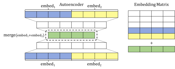
3. Autoencoder: Train a small network to predict the two items’ embeddings, given those embeddings. The middle hidden layer should be the size of only one embedding. After training the network, this value is used as the new, merged item’s embedding. This one works best.

The authors use standard datasets (WMT and IWSLT) for training from English into a morphologically rich language: Czech or German. They found that optimal performance on smaller datasets may come from fewer subword units, and that the same number of units wouldn’t be optimal across datasets.

Their incremental approach would typically underestimate the optimal vocabulary size from the grid search, but the performance beats the sweep result with the same vocabulary size.

Altogether, an interesting and useful paper with the message that fixing a hyperparameter is a bad idea. The fact that it can be effectively tuned inline during training is especially impressive.

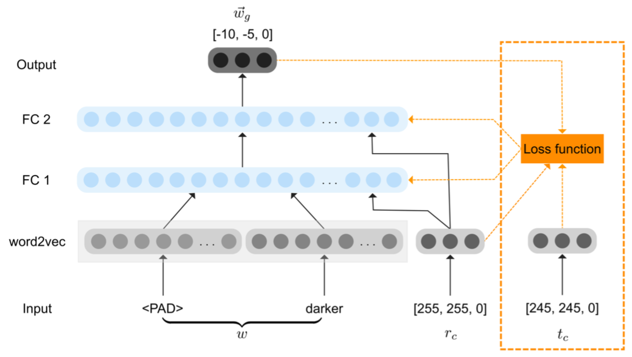
When naming a target color that is similar to a distractor, we use comparative adjectives (Monroe et al., 2017). This relates to the notion of codability, or entropy: it takes more bits to distinguish between the two colors, because our broad-level categories don’t manage to distinguish them. The work of Winn and Muresan seeks to ground these comparisons. They want to match each descriptor up to a vector, transforming “blue” + “lighter (given that the color is blue)” = “lighter blue”.

The authors used the data of the xkcd color survey, which elicited 954 color names from 500 namings and 222,500 user sessions. Many of these were compositional (though not comparative), and each label had on average 600 datapoints. (Sure, but what’s the distribution? No doubt ‘red’ was way more common than ‘filemot’.) Winn and Muresan distilled the data down to 415 tuples like (ʙʟᴜᴇ, ‘lighter’, ʟɪɢʜᴛ ʙʟᴜᴇ), where ʙʟᴜᴇ actually is a set of RGB datapoint. There are 79 unique reference labels (like ʙʟᴜᴇ) and 81 unique comparatives—relatively slim pickings.

The authors make a poor assumption: that you can simply compare the averages of the sets to learn the positions. With that, all you’d need is to average each cluster and compute a vector from centroid to centroid. :-/

Hey, while we’re on silly things that this (somehow) ACL best paper did—RGB coordinates were used in the data collection, sure, but using them to find the vectors encoding the comparatives is relatively meaningless—the distances in RGB space don’t align with perceptual judgments of similarity.

Aaaand now for some reason, since this is an ACL paper, we have to work Word Embeddings into it. We evidently use these to condition our vector on the input word. This is what gives the model an ability to predict new vectors. (But this assumes you a priori know the general category labels and their coordinates.)

The bottom line

Nobody has done work on grounding comparatives before, the authors contend. But isn’t a comparative only meaningful in the context of a reference color, so we open the door to massive overfitting. This paper feels like a fun blog post, and I’m sure the color and examples made it eye-catching. But there’s not a whole lot of meat to it.

Before the age of neural MT, post-editing generally was a phrase-based MT process. An automatically produced alignment would help create a new, “source-context aware”, source text. It would have the tokens of the MT output and the tokens of the original source paired together.

This paper, leaping into the neural age, builds on the standard model (plus a few additions made in the Nematus toolkit—the decoder is wonky, using GRUs out the wazoo). They introduce four model variants. To understand them, we should understand the difference between hard and soft attention. Soft attention means that multiple encoder states can make fractional contributions to picking the output token of the decoder. Hard attention makes you rely on only one state per output token. It’s like the relationship between k-means and a Gaussian mixture model.

1. Hard, monotonic attention. This borrows from Aharoni and Goldberg’s system for morphological inflection—another string transduction task. The system can predict not only a word, but also a special symbol <STEP> which forces the attention mechanism to advance to the next encoder state. To precompute the <STEP> tokens interleaved into the input, the authors use the Longest Common Subsequence between the MT output and the correct translation.
2. Hard and soft attention. Hard attention meant swapping out the decoder for something without the standard attention mechanism. What if we brought it back? Append the hard attention’s encoder state to the standard (soft) attention’s state.
3. Soft dual-attention. This is the idea of Zoph and Knight, but expressed more clearly. Let’s compute standard attention over both the source (which was previously unused) and the MT output—each from separate encoders—then concatenate those.
4. Hard attention with soft dual-attention. Strap two of those hard-and-soft mechanisms together.

The authors followed the conventions of the 2016 WMT shared task on automatic post-editing, including evaluation by Translation Edit Rate (TER), with the widespread BLEU as only a secondary metric.

They also performed model averaging—taking the best 8 checkpoints from the training process. This regularization, they found, improved performance.

Enough about their experimental framework. Let’s dig into error analysis.

They found that their models chose to edit 75–80% of the sentences, no matter what. The majority were improved, while about a quarter of the edited sentences were deteriorated.

The authors present visualizations of their attention matrices.

For CGRU-HARD [hard and soft dual-attention], it is interesting to see how the monotonic attention now allows the soft attention mechanism to look around the input sentence more freely or to remain inactive instead of following the monotonic path.

TLDR: Use both sequences for APE. Dual attention over both the original source and the MT output that needs editing does better than just editing the output while ignoring the source.

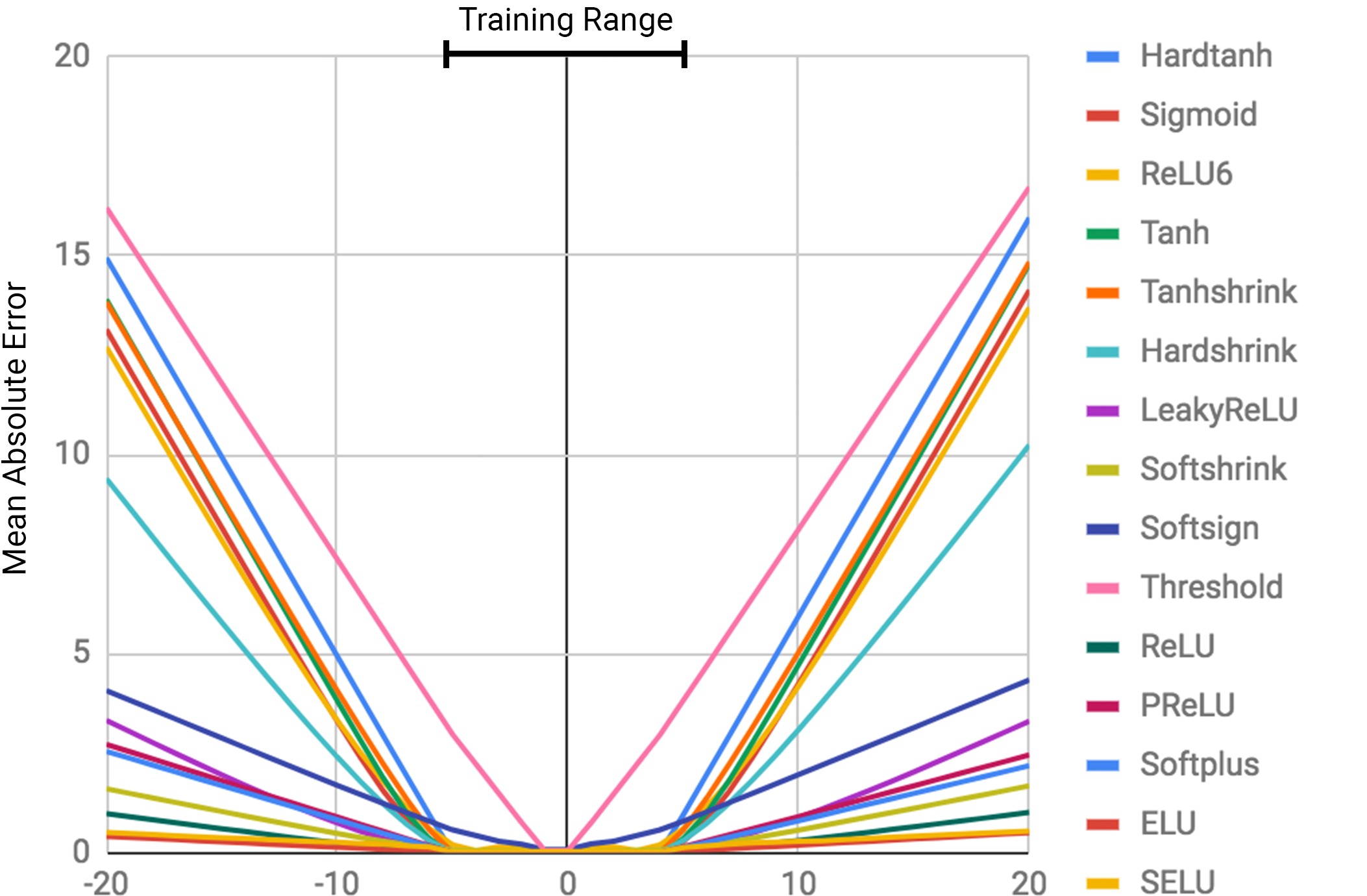
Neural networks have trouble with things as simple to us as learning the identity function \(f(x) = x\). Within the numerical range they’re trained on, they do fine, but they can’t extrapolate.

The paper proposes two new models that generalize better. The first, for better addition and subtraction, is the neural accumulator (NAC). It’s like a normal linear layer, but there’s no bias, and its weight matrix \(\mathbf{W}\) is only 0’s, 1’s, and −1’s. Well, sort of. Hard constraints are not differentiable. Instead, they express \( \mathbf{W} = \tanh(\mathbf{\hat{W}}) \odot \sigma(\mathbf{\hat{M}}) \). The tanh values range from -1 to 1, the sigmoid ranges from 0 to 1, and the values of both are strongly encouraged toward the extremes, so each element-wise product is pushed to the values we want.

The second is a neural arithmetic logic unit (NALU), christened after the structures you remember from your computer architecture classes. It combines two of these NACs, one of which operates in log-space, so it can perform multiplication and division. (\(\exp(\log(a) + \log(b)) \equiv a \times b\).) A gate controls whether the NALU takes the add/subtract route or the multiply/divide route.

Their results show that normal neural architectures do poorly at generalizing, even if they can handle the simple addition and subtraction. The NAC does just as well, but the NALU is the only variant that learns to extrapolate beyond the range of training values. When the values are fed in sequentially (rather than as one vector), the LSTM and ReLU-activated RNN both learn interpolation, but fail at extrapolation. NALU learns most extrapolation, but it fails miserably on division. (They justify this by the fact that small denominators can tease out the error in generalization ability.)

They also test performance on two other tasks: MNIST digit counting and digit adding. Both involve recognizing images of digits, then using them. (Digit counting involves a swarm of numbers in each picture.) The NAC (designed for addition and subtraction) wins at this. It’s easily incorporated into existing image recognition architectures by replacing the final layer.

Another task is interpreting text representations of numbers, turning them into text. Here, the NALU shines.

The takeaway:

• We have a single ‘neuron’ that can better handle math.
• It’s easily integrable into existing image classification networks or text interpretation.

To help our models out, we want to make the source text more similar to the target.

Shearing et al.’s innovation is the inclusion of morphological glosses, which makes dictionaries more useful. Dictionaries often list only a principal form for a set of words: “run” but not “running” or “ran”. The authors’ glossing process creates in-place translations of “running” and “ran” from the one for “run” and knowledge about verb tense.

The morphological glosses work into a four-stage pipeline that creates an out-of-order English (English-prime; \(E’\)) from the foreign source text. For each foreign word, do the following:

1. Analyze the word to get a lemma and morphological tag: comprábamos → comprar, V;1;PL;PST;IPFV
2. Look up the lemma in a lemma-to-lemma dictionary: comprar → buy
3. Convert the morphological features into a morphological gloss: V;1;PL;PST;IPFV → ‘(we) were VBG.’
4. Replace the placeholder (VBG) with the corresponding form of the English lemma: ‘(we) were VBG’ + buy → ‘(we) were buying’

At the end, you get comprábamos → ‘(we) were buying’, which the authors stick into a phrase-based translation model, turning \(E’\) into \(E\).

Little details:

• Morph analysis using Kann and Schütze (2016).
• Translate lemmas with PanLex or Wiktionary.
• Manually create glosses.
• Inflect English with Spedt and Daelemans (2012).
• The LORELEI data they use gives multiple definitions for some words. Split these into separate lines, expanding your Bitext.
• Append a gloss-to-gloss identity mapping to the bitext, biasing the aligner toward lining these two up.