<?xml version="1.0" encoding="utf-8"?><feed xmlns="http://www.w3.org/2005/Atom" ><generator uri="https://jekyllrb.com/" version="3.10.0">Jekyll</generator><link href="https://anie.me/feed.xml" rel="self" type="application/atom+xml" /><link href="https://anie.me/" rel="alternate" type="text/html" /><updated>2026-08-18T01:36:39+00:00</updated><id>https://anie.me/feed.xml</id><title type="html">Allen Nie</title><subtitle>A blog for RL, NLP, and Programming</subtitle><entry><title type="html">On Bias and Variance Decomposition of Offline Policy Evaluation Estimators</title><link href="https://anie.me/bias-variance-of-ope/" rel="alternate" type="text/html" title="On Bias and Variance Decomposition of Offline Policy Evaluation Estimators" /><published>2025-01-10T00:00:00+00:00</published><updated>2025-01-10T00:00:00+00:00</updated><id>https://anie.me/bias-variance-of-ope</id><content type="html" xml:base="https://anie.me/bias-variance-of-ope/"><![CDATA[<p>Note: This blog post is an unpublished partial draft of a larger work, jointly written with <a href="https://aishwaryamandyam.com/">Aishwarya Mandyam</a>.</p>

<h2 id="introduction">Introduction</h2>

<p>Evaluation is a critical component of learning contextual bandit policies that can be deployed in high-risk settings. One way to perform this evaluation is to directly deploy it in the setting of interest, or use an accurate simulator evaluate how well this policy will do when deployed. Unfortunately, directly deploying this policy may be unsafe or unethical (i.e. deploying in a hospital environment), and we may not have accurate simulators of the deployment setting. In this case, we turn to Off-policy Evaluation (OPE), which estimates the value of the learned policy using an offline or cached dataset of samples that arise from a behavior policy. The challenge is that this behavior policy is distinct from the target policy, and there may be limited coverage of the behavior dataset in areas of the state-action space where the target policy frequents. Several strategies have been proposed to mitigate this dataset distribution shift.</p>

<h2 id="categories-of-ope-estimators">Categories of OPE estimators</h2>

<p>There are three broad categories of OPE estimators. The first is the direct method (DM)[1], which in the contextual bandit setting, approximates the reward function, and uses that reward model to simulate the target policy. Typically, if the reward function estimate is good (as in the reward model is fully realizable, and there is enough data to estimate it), DM is a great option for OPE. When the reward estimate is bad, DM estimators typically have high bias.</p>

<p>The second option is importance sampling (IS)[2], in which you re-weight samples in the behavior dataset as if they appeared from the target policy. The weight used is an importance sampling ratio, typically written as $\rho$, which compares how likely a sample is to occur in the target policy and the behavior policy. IS-based OPE estimators typically have high variance.</p>

<h2 id="notation">Notation</h2>

<p>$\pi_e$ : target, or learned policy. Our goal is to evaluate this policy.</p>

<p>$\pi_b$ : behavior policy. Our offline dataset contains samples that arise from this behavior policy.</p>

<p>$\rho = \frac{\pi_e(a \vert s)}{\pi_b(a \vert s)}$ : importance sampling ratio comparing the likelihood of observing a sample in the target policy to the likelihood of observing it in the behavior policy</p>

<p>$S,A$ : state and action spaces</p>

<p>$s, a, r$ : observed state, action, and reward</p>

<p>$N$: number of samples</p>

<p>$d$ : state distribution</p>

<p>$R(s,a)$: the true reward function used for the factual dataset, with mean $\bar{R}(s,a)$ and variance $\sigma^2(s,a)$.</p>

<p>$D_1 \sim \mathcal{D}$: dataset used to fit the OPE estimate</p>

<p>$D_{\hat{R}} \sim \mathcal{D}$: dataset used to fit the reward model</p>

<p>$V = V(\pi_e) = \mathbb{E}_{s \sim  d, a\sim\pi_e}[R(s, a)]$: the true return of the model. $\hat V$ is an estimator for this estimand.</p>

<h2 id="direct-method">Direct Method</h2>

<p>The direct method is  $\hat{V}^{DM} = \frac{1}{N}\sum_{i=1}^N \sum_{a \in A}\pi_e(a \vert s_i) \hat{R}(s_i, a_i)$.</p>

<h3 id="bias-derivation">Bias Derivation</h3>

<p>First we use the linearity of expectation and definition of expectation over $D_1$. Then, we use the mean of the distribution $R$. Finally, we use the definition of the value function and the policy value.</p>

<pre>
\begin{align}\mathbb{E}_{D_1 \sim\mathcal{D}, D_{\hat{R}} \sim \mathcal{D}}[\hat{V}^{\text{DM}}] &amp;= \mathbb{E}_{D_1 \sim\mathcal{D}} \mathbb{E}_{D_{\hat{R}} \sim \mathcal{D}} \left[ \frac{1}{N}\sum_{s_i \in D_1} \sum_{a \in A} \pi_e(a|s_i) \hat{R}(s_i,a) \right] \\
&amp;= \mathbb{E}_{D_1 \sim \mathcal{D}} \left[ \frac{1}{N} \sum_{j=1}^{N} \sum_{a \in A} \pi_e(a|s_i) \mathbb{E}_{D_{\hat{R}} \sim \mathcal{D}} [\hat{R}(s_i,a) ] \right] \\
&amp;= \frac{1}{N} \sum_{i=1}^{N} \mathbb{E}_{D_1 \sim\mathcal{D}} \left[ \sum_{a \in A} \pi_e(a|s_i) \mathbb{E}_{D_{\hat{R}} \sim \mathcal{D}} [\hat{R}(s_i,a) ] \right] \\
&amp;= \frac{1}{N} \sum_{i=1}^{N} \sum_{s \in \mathcal{S}} d(s) \left( \sum_{a \in A} \pi_e(a|s) \mathbb{E}_{D_{\hat{R}} \sim \mathcal{D}} [\hat{R}(s,a) ] \right) \\
&amp;= \frac{1}{N} \sum_{i=1}^{N} \sum_{s \in \mathcal{S}} d(s) \left( \sum_{a \in A} \pi_e(a|s) \bar{R}(s,a) \right) \\
&amp;= \frac{1}{N} \sum_{i=1}^{N} \sum_{s \in \mathcal{S}} d(s) V^{\pi_e}(s_i) \\
&amp;= \frac{1}{N} \sum_{i=1}^{N} V(\pi_e) \\
&amp;= V(\pi_e)\end{align}
</pre>

<h3 id="variance-derivation">Variance Derivation</h3>

<p>By law of total variance, we can decompose the variance of the direct method estimator into two terms:</p>

<pre>
\begin{align}
&amp; \mathbb{V}_{D_{\hat{R}} \sim\mathcal{D}, D_{1} \sim \mathcal{D}}[\hat{V}^{\text{DM}}] = \underbrace{\mathbb{V}_{D_{\hat{R}} \sim\mathcal{D}} \mathbb{E}_{D_{\hat{R}} \sim \mathcal{D}} \left[\hat{V}^{\text{DM}}\right]}{(1)} + \underbrace{\mathbb{E}_{D_{\hat{R}} \sim\mathcal{D}} \mathbb{V}_{D_{\hat{R}} \sim \mathcal{D}} \left[ \hat{V}^{\text{DM}} \right]}_{(1')}
\end{align}
</pre>

<p>We can substitute the intermediate result from the proof of the bias of DM into (1):</p>

<pre>
\begin{align}
(1) &amp;= \mathbb{V}_{D_{\hat{R}} \sim\mathcal{D}} \left[ \mathbb{E}_{D_{\hat{R}} \sim \mathcal{D}}\big[ \hat{V}^{\text{DM}} \big] \right] = \mathbb{V}_{D_{\hat{R}} \sim\mathcal{D}} \left[ \hat{R}(d_0,\pi_e) \right]
\end{align}
</pre>

<p>For (1’), we first consider the inner variance with respect to $D_{\hat{R}}$ assuming $\hat{R}$ is given:</p>

<pre>
\begin{align}
\mathbb{V}_{D_{\hat{R}} \sim \mathcal{D}} \left[ \hat{V}^{\text{DM}} \right] &amp;= \mathbb{V}_{D_{\hat{R}} \sim \mathcal{D}} \left[ \frac{1}{N} \sum_{i=1}^{N} \sum_{a \in A} \pi_e(a|s_i) \hat{R}(s_i,a) \right] \\
&amp;= \frac{1}{N^2} \sum_{i=1}^{N} \mathbb{V}_{s_i \sim d_0} \left[ \hat{R}(s_i,\pi_e) \right] \\
&amp;= \frac{1}{N} \mathbb{V}_{s \sim d_0} \left[ \hat{R}(s,\pi_e) \right]
\end{align}
</pre>

<p>Substituting this into (1’):</p>

<pre>
\begin{align}
&amp; (1') = \mathbb{E}_{D_{\hat{R}} \sim\mathcal{D}} \mathbb{V}_{D_{\hat{R}} \sim \mathcal{D}} \left[ \hat{V}^{\text{DM}} \right] \\
&amp;= \mathbb{E}_{D_{\hat{R}} \sim\mathcal{D}} \left[ \frac{1}{N} \mathbb{V}_{s \sim d_0} \left[ \hat{R}(s,\pi_e) \right] \right] \\
&amp;= \frac{1}{N} \mathbb{E}_{D_{\hat{R}} \sim\mathcal{D}} \left[ \mathbb{E}_{s \sim d_0} \left[ \hat{R}(s,\pi_e)^2 \right] - \mathbb{E}_{s \sim d_0} \left[ \hat{R}(s,\pi_e) \right]^2 \right]  &amp;&amp; \\
&amp;= \frac{1}{N} \Bigg( \underbrace{\mathbb{E}_{D_{\hat{R}} \sim\mathcal{D}} \mathbb{E}_{s \sim d_0} \left[ \hat{R}(s,\pi_e)^2 \right]}_{(2)} - \underbrace{\mathbb{E}_{D_{\hat{R}} \sim\mathcal{D}}\left[\mathbb{E}_{s \sim d_0} \left[ \hat{R}(s,\pi_e) \right]^2 \right]}_{(2')} \Bigg)
\end{align}
</pre>

<pre>
\begin{align}
(2) &amp;= \mathbb{E}_{D_{\hat{R}} \sim\mathcal{D}} \mathbb{E}_{s \sim d_0} \left[ \hat{R}(s,\pi_e)^2 \right] \\
&amp;= \mathbb{E}_{s \sim d_0} \mathbb{E}_{D_{\hat{R}} \sim\mathcal{D}} \left[ \hat{R}(s,\pi_e)^2 \right] \\
&amp;= \mathbb{E}_{s \sim d_0} \left[ v^{\pi_e}(s)^2 + \mathbb{V}_{D_{\hat{R}}\sim\mathcal{D}}[\hat{R}(s,\pi_e)] \right] \\
&amp;= \mathbb{E}_{s \sim d_0} \left[ {v^{\pi_e}(s)}^2 \right] + \mathbb{E}_{s \sim d_0} \left[ \mathbb{V}_{D_{\hat{R}} \sim\mathcal{D}} [ \hat{R}(s,\pi_e) ] \right] \\
&amp;= \mathbb{E}_{s \sim d_0} \left[ {v^{\pi_e}(s)} \right]^2 + \mathbb{V}_{s \sim d_0} \left[ {v^{\pi_e}(s)} \right] + \mathbb{E}_{s \sim d_0} \left[ \mathbb{V}_{D_{\hat{R}} \sim\mathcal{D}} [ \hat{R}(s,\pi_e) ] \right] &amp;&amp;  \\
&amp;= {v(\pi_e)}^2 + \mathbb{V}_{s \sim d_0} \left[ {v^{\pi_e}(s)} \right] + \mathbb{E}_{s \sim d_0} \left[ \mathbb{V}_{D{\hat{R}} \sim\mathcal{D}} [ \hat{R}(s,\pi_e) ] \right]  \\
\\
(2') &amp;= \mathbb{E}_{D_{\hat{R}} \sim\mathcal{D}}\left[\mathbb{E}_{s \sim d_0} \left[ \hat{R}(s,\pi_e) \right]^2 \right] \\
&amp;= \mathbb{E}_{D_{\hat{R}} \sim\mathcal{D}}\left[\hat{R}(d_0,\pi_e)^2 \right] \\
&amp;= v(\pi_e)^2 + \mathbb{V}_{D_{\hat{R}}\sim\mathcal{D}}[\hat{R}(d_0,\pi_e)]
\end{align}
</pre>

<p>Thus,</p>

<pre>
\begin{align}
(2) - (2') &amp;= \mathbb{V}_{s \sim d_0} \left[ {v^{\pi_e}(s)} \right] + \mathbb{E}_{s \sim d_0} \left[ \mathbb{V}_{D_{\hat{R}} \sim\mathcal{D}} [ \hat{R}(s,\pi_e) ] \right] - \mathbb{V}_{D_{\hat{R}} \sim\mathcal{D}}\left[\hat{R}(d_0,\pi_e) \right] \\
\end{align}
</pre>

<p>Putting everything together, we have:</p>

<pre>
\begin{align}
&amp; \mathbb{V}_{D_{\hat{R}} \sim\mathcal{D}, D_{\hat{R}} \sim \mathcal{D}}[\hat{V}^{\text{DM}}] = (1) + (1') \\
&amp;= \mathbb{V}_{D_{\hat{R}} \sim\mathcal{D}} \left[ \hat{R}(d_0,\pi_e) \right] \\
&amp;+ \frac{1}{N} \left(\mathbb{V}_{s \sim d_0} \left[ {v^{\pi_e}(s)} \right] + \mathbb{E}_{s \sim d_0} \left[ \mathbb{V}_{D{\hat{R}} \sim\mathcal{D}} [ \hat{R}(s,\pi_e) ] \right] - \mathbb{V}_{D_{\hat{R}} \sim\mathcal{D}}\left[\hat{R}(d_0,\pi_e) \right]\right) \\
&amp;= \frac{1}{N}\mathbb{V}_{s \sim d_0} \left[ {v^{\pi_e}(s)} \right] + \frac{1}{N}\mathbb{E}_{s \sim d_0} \left[ \mathbb{V}_{D_{\hat{R}} \sim\mathcal{D}} [ \hat{R}(s,\pi_e) ] \right] + \big(1-\frac{1}{N}\big) \mathbb{V}_{D_{\hat{R}} \sim\mathcal{D}}\left[\hat{R}(d_0,\pi_e) \right] \\
&amp;= \frac{1}{N}\mathbb{V}_{s \sim d_0} \left[ {v^{\pi_e}(s)} \right] \frac{1}{N}\mathbb{E}_{s \sim d_0} \bigg[ \mathbb{E}_{a \sim \pi_e} \Big[\pi_e(a|s) \, \sigma_R^2(s,a) \, \mathbb{E}_{D{\hat{R}} \sim \mathcal{D}}\big[\frac{1}{N_{s,a}(D_{\hat{R}})}\big] \Big] \bigg] \\
&amp; \qquad \qquad \qquad \qquad \;\; + \big(1-\frac{1}{N}\big) \mathbb{E}_{s \sim d_0}\mathbb{E}_{a \sim \pi_e} \left[d_0(s) \, \pi_e(a|s) \, \sigma_R^2(s,a) \, \mathbb{E}_{D_{\hat{R}} \sim \mathcal{D}}\Big[\frac{1}{N_{s,a}(D_{\hat{R}})}\Big] \right] \\
&amp;= \frac{1}{N}\mathbb{V}_{s \sim d_0} \left[ {v^{\pi_e}(s)} \right] \\
&amp;+ \mathbb{E}_{s \sim d_0}\mathbb{E}_{a \sim \pi_e} \left[\Big(\frac{1}{N} + \big(1-\frac{1}{N}\big)d_0(s) \Big) \, \pi_e(a|s) \, \sigma_R^2(s,a) \, \mathbb{E}_{D_{\hat{R}} \sim \mathcal{D}}\Big[\frac{1}{N_{s,a}(D_{\hat{R}})}\Big] \right]
\end{align}
</pre>

<h2 id="importance-sampling">Importance Sampling</h2>

<p>The importance sampling (IS) estimator is: $\hat V^{\text{IS}} = \frac{1}{N}\sum_{i=1}^N \frac{\pi_e(a_i \vert s_i)}{\pi_b(a_i \vert s_i)} r_i$</p>

<h2 id="bias-derivation-1">Bias Derivation</h2>

<p>Importance sampling estimator is unbiased.</p>

<pre>
\begin{align}\mathbb{E}_{D \sim \mathcal{D}}[\hat V^{\text{IS}}] &amp;= \mathbb{E}_{s_i \sim d, a_i \sim \pi_b} \Bigg[\frac{1}{N}\sum_{i=1}^N \frac{\pi_e(a_i|s_i)}{\pi_b(a_i|s_i)} r_i \Bigg] \\
&amp;= \frac{1}{N}\sum_{i=1}^N \mathbb{E}_{s_i \sim d, a_i \sim \pi_b} \Bigg[ \frac{\pi_e(a_i|s_i)}{\pi_b(a_i|s_i)} r_i \Bigg] \\
&amp;= \frac{1}{N}\sum_{i=1}^N \mathbb{E}_{s_i \sim d} \Bigg[ \pi_b(a_i|s_i) \frac{ \pi_e(a_i|s_i)}{\pi_b(a_i|s_i)} r_i \Bigg] \\
&amp;= \frac{1}{N}\sum_{i=1}^N \mathbb{E}_{s_i \sim d} \Bigg[  \pi_e(a_i|s_i) r_i \Bigg] \\
&amp;= \frac{1}{N}\sum_{i=1}^N \mathbb{E}_{s_i \sim d, a_i \sim \pi_e(s_i)} \Big[ r_i \Big] \\
&amp;= \frac{1}{N}\sum_{i=1}^N V(\pi_e) \\
&amp;= V(\pi_e)
\end{align}
</pre>

<h2 id="variance-derivation-1">Variance Derivation</h2>

<p>However, Importance sampling estimator is known for having a relatively large variance.</p>

<pre>
\begin{align}
\mathbb{V}_{D \sim \mathcal{D}}[\hat{V}^{\text{IS}}] &amp;= \mathbb{V}_{s_i \sim d, a_i \sim \pi_b} \Bigg[ \frac{1}{N}\sum_{i=1}^N \frac{\pi_e(a_i|s_i)}{\pi_b(a_i|s_i)} R(s_i, a_i) \Bigg] \\
&amp;= \frac{1}{N^2} \mathbb{V}_{s_i \sim d, a_i \sim \pi_b} \Bigg[ \sum_{i=1}^N \frac{\pi_e(a_i|s_i)}{\pi_b(a_i|s_i)} R(s_i, a_i) \Bigg] \\
&amp;= \frac{1}{N} \mathbb{V}_{s_i \sim d, a_i \sim \pi_b} \Bigg[  \frac{\pi_e(a_i|s_i)}{\pi_b(a_i|s_i)} R(s_i, a_i) \Bigg]\\
\end{align}
</pre>

<p>Step 24 to 25 is because we know each sample is i.i.d. Let $w_i = \frac{\pi_e(a_i \vert s_i)}{\pi_b(a_i \vert s_i)}$, the <strong>empirical variance estimator</strong> is:</p>

<pre>
$$
\hat{\mathbb{V}}_{D \sim \mathcal{D}}[\hat{V}^{\text{IS}}] = \frac{1}{N} \sum_{i=1}^N \big (w_i R(s_i, a_i) - \hat V^{\text{IS}} \big)^2
$$
</pre>

<h3 id="bonus-content-weighted-importance-sampling">Bonus Content (Weighted Importance Sampling)</h3>

<p>Weighted importance sampling estimator is also called a self-normalizing importance sampling estimator. It is a biased estimator but has smaller variance compared to IS.</p>

<p>WIS can be defined as (using $w_i = \frac{\pi_e(a_i \vert s_i)}{\pi_b(a_i \vert s_i)}$)</p>

<pre>
$$
\hat V^{\text{WIS}} = \frac{\sum_{i=1}^N w_i R(s_i, a_i)}{\sum_{i=1}^N w_i} = \sum_{i=1}^N \frac{w_i}{\sum_{i=1}^N w_i} R(s_i, a_i)
$$
</pre>

<p>We show a quick derivation of their bias and variance.</p>

<p><strong>Bias Derivation</strong></p>

<pre>
\begin{align}\mathbb{E}_{D \sim \mathcal{D}}[\hat V^{\text{WIS}}] &amp;= \mathbb{E}_{s_i \sim d, a_i \sim \pi_b} \Bigg[\sum_{i=1}^N \frac{w_i}{\sum_{i=1}^N w_i} R(s_i, a_i) \Bigg] \\
&amp;= \sum_{i=1}^N \mathbb{E}_{s_i \sim d, a_i \sim \pi_b} \Bigg[ \frac{w_i}{\sum_{i=1}^N w_i} R(s_i, a_i) \Bigg] \\
&amp;= \sum_{i=1}^N \frac{1}{\mathbb{E}_{s_i \sim d, a_i \sim \pi_b} [\sum_{i=1}^N w_i]} \mathbb{E}_{s_i \sim d, a_i \sim \pi_b} \Bigg[ w_i R(s_i, a_i) \Bigg] \\
&amp;=\sum_{i=1}^N \frac{1}{\sum_{i=1}^N\mathbb{E}_{s_i \sim d, a_i \sim \pi_b} [w_i]} \mathbb{E}_{s_i \sim d, a_i \sim \pi_b}\Bigg[ \frac{\pi_e(a_i|s_i)}{\pi_b(a_i|s_i)} R(s_i, a_i) \Bigg] \\
&amp;=\sum_{i=1}^N \frac{1}{\sum_{i=1}^N\mathbb{E}_{s_i \sim d, a_i \sim \pi_b} [w_i]} V(\pi_e) \\
&amp;= \frac{1}{\sum_{i=1}^N\mathbb{E}_{s_i \sim d, a_i \sim \pi_b} [w_i]} \sum_{i=1}^N V(\pi_e)
\end{align}
</pre>

<p>Step (29) to step (30) followed the IS bias derivation. We can see that WIS estimator is only unbiased when</p>
<pre>$\sum_{i=1}^N\mathbb{E}_{s_i \sim d, a_i \sim \pi_b} [w_i] = N$,</pre>
<p>which means $\mathbb{E}_{s_i \sim d, a_i \sim \pi_b} [w_i] = 1$. If the evaluation policy $\pi_e$ and behavior policy $\pi_b$ takes the exact same action, then this estimator is unbiased.</p>

<p><strong>Consistency Corollary</strong></p>

<p>This is a biased estimator</p>

<pre>
$$
\hat V^{\text{WIS}}  =  \underbrace{\frac{1}{\frac{1}{N}\sum_{i=1}^N w_i}}_{a} \cdot \underbrace{\frac{1}{N} \sum_{i=1}^N  w_iR(s_i, a_i)}_{b}
$$
</pre>

<p>We can show that $\hat V^{\text{WIS}}$ is consistent.</p>

<pre>
$$
\lim_{N \rightarrow \infty }\frac{1}{N}\sum_{i=1}^N w_i \stackrel{a.s.}{\rightarrow} \mathbb{E}_{s_i \sim d, a_i \sim \pi_b} \Big[ \frac{\pi_e(a_i|s_i)}{\pi_b(a_i|s_i)} \Big] = \mathbb{E}_{s_i \sim d} \Big[ \pi_e(a_i|s_i)\Big] = 1
$$
</pre>

<p>As we can see, $a \rightarrow 1$ as $N \rightarrow \infty$. We can also apply the strong law of large numbers on $b$ and see $b \rightarrow V(\pi_e)$ as $N \rightarrow \infty$.  Therefore, $\hat V^{\text{WIS}} \rightarrow V(\pi_e)$ as $N \rightarrow \infty$.</p>

<p><strong>Variance Derivation</strong></p>

<p>Variance of an WIS estimator requires derivation over $\frac{w_i}{\sum_{i}w_i}$, which in its essence, a ratio — the variance of this ratio through the sampled dataset $D$ has an effect on the overall variance of WIS. In order to work this part out, we will first very quickly discuss the multivariate delta method:</p>

<p>For ease of discussion, we define two dummy variables $X = \frac{1}{N} \sum_{i} w_i R(s_i, a_i)$ and $Y = \frac{1}{N} \sum_i w_i$. It’s easy to see $\hat V^{\text{WIS}} = X/Y$. Let $\mu_x = \mathbb{E}[X]$ and $\mu_y = \mathbb{E}[Y]$. We can define a two-variable function $f(x, y) = x/y$ and its first-order Taylor Expansion to be:</p>

<pre>
$$
f(X, Y) \approx f(\mu_x, \mu_y) + \nabla_X f(\mu_x, \mu_y)(X - \mu_x) + \nabla_Y f(\mu_x, \mu_y)(Y-\mu_y)
$$
</pre>

<p>If we take variance on both side, we get:</p>

<pre>
$$
\mathbb{V}_{D \sim \mathcal{D}} \Bigg[\frac{X}{Y} \Bigg] \approx \Big(\nabla_X f(\mu_x, \mu_y) \Big)^2 \mathbb{V}[X] + \Big(\nabla_Y(\mu_x, \mu_y) \Big)^2 \mathbb{V}[Y] + 2 \nabla_X f(\mu_x, \mu_y) \nabla_Y f(\mu_x, \mu_y) \mathrm{Cov}(X, Y)
$$
</pre>

<p>Note that $\nabla_X f = \frac{1}{Y}$, therefore, $\nabla_X f(\mu_x, \mu_y) = \frac{1}{\mu_y}$. Similarly, $\nabla_Y f = \frac{X}{Y^2}$, therefore $\nabla_Y f(\mu_x, \mu_y) = \frac{\mu_x}{\mu_y^2}$. Using that, we can write out the equation above as below. We also assume $w_i \sim W, R(s_i, a_i) \sim R$ (where both $W$ and $R$ have randomness over $D$).</p>

<pre>
\begin{align}
\mathbb{V}_{D \sim \mathcal{D}}\Bigg[\frac{X}{Y} \Bigg] &amp;\approx \frac{1}{\mu_x^2}\frac{1}{N}\mathbb{E}\Big[(WR - \mu_x)^2 \Big] + \frac{\mu_x^2}{\mu_y^4} \frac{1}{N} \mathbb{E} \Big[(W - \mu_y)^2 \Big] \\ &amp;- 2\frac{1}{\mu_y} \frac{\mu_x}{\mu_y^2} \mathbb{E} \Big[W^2 R \Big] + 2 \frac{1}{\mu_y} \frac{\mu_x}{\mu_y^2} \mathbb{E} \Big[WR \Big] \mathbb{E} \Big[W \Big] \\
&amp;=\frac{1}{\mu_y^2} \frac{1}{N} \Bigg[ \mathbb{E} \Big[ W^2 R^2\Big] + \frac{\mu_x^2}{\mu_y^2} \Big[ W^2\Big] - 2 \frac{\mu_x}{\mu_y} \mathbb{E} \Big[ W^2 R\Big] \Bigg] \\
&amp;= \frac{1}{\mu_y^2} \frac{1}{N} \mathbb{E} \Big[ (WR - \frac{\mu_x}{\mu_y}W)^2\Big] \\
&amp;= \frac{1}{N} \frac{\mathbb{E} \Big[ W^2 (R - \frac{\mu_x}{\mu_y})^2 \Big]}{\mu_y^2}
\end{align}
</pre>

<p>Note that $\mu_x / \mu_y = V^{\text{WIS}}$, therefore, we can write this as:</p>

<pre>
$$
\mathbb{V}_{D \sim \mathcal{D}} [\hat V^{\text{WIS}}] \approx \frac{1}{N}\frac{\mathbb{E}_{D \sim \mathcal{D}} \Bigg[ w_i^2 \Big(R(s_i, a_i) - \hat V^{\text{WIS}} \Big)^2 \Bigg]}{\mathbb{E}_{D \sim \mathcal{D}}\big[w_i \big]^2}
$$
</pre>

<p>The empirical variance estimator for this is:</p>

<pre>
\begin{align}
\hat{\mathbb{V}}_{D \sim \mathcal{D}}[\hat V^{\text{WIS}}] &amp;= \frac{1}{N} \frac{\frac{1}{N} \sum_{i=1}^N w_i^2 \Big(R(s_i, a_i) - \hat V^{\text{WIS}} \Big)^2 }{(\frac{1}{N} \sum_{i=1}^N w_i)^2} \\
&amp;= \sum_{i=1}^N \Big(\frac{w_i}{\sum_{i=1}^N w_i}\Big)^2 \Big( R(s_i, a_i) - \hat V^{\text{WIS}} \Big)^2
\end{align}
</pre>

<p>Note that unlike other variance estimator, we do not have the $1/N$ term after summation.</p>

<p>Reference: <a href="https://www.stat.cmu.edu/~hseltman/files/ratio.pdf">https://www.stat.cmu.edu/~hseltman/files/ratio.pdf</a></p>]]></content><author><name></name></author><summary type="html"><![CDATA[Note: This blog post is an unpublished partial draft of a larger work, jointly written with Aishwarya Mandyam.]]></summary></entry><entry><title type="html">Grading Complex Interactive Coding Programs with Reinforcement Learning</title><link href="https://anie.me/play2grade/" rel="alternate" type="text/html" title="Grading Complex Interactive Coding Programs with Reinforcement Learning" /><published>2022-03-26T00:00:00+00:00</published><updated>2022-03-26T00:00:00+00:00</updated><id>https://anie.me/play2grade</id><content type="html" xml:base="https://anie.me/play2grade/"><![CDATA[<p><strong>[Summary] tl;dr:</strong> A tremendous amount of effort has been poured into training AI algorithms to competitively play games that computers have traditionally had trouble with, such as the retro games published by Atari, Go, DotA, and StarCraft II. The practical machine learning knowledge accumulated in developing these algorithms  has paved the way for people to now routinely train game-playing AI agents for many games. Following this line of work, we focus on a specific category of games – those developed by students as part of a programming assignment.  Can the same algorithms that master Atari games help us grade these game assignments? In our recent NeurIPS 2021 <a href="https://arxiv.org/abs/2110.14615">paper</a>, we illustrate the challenges in treating interactive coding assignment grading as game playing and introduce the Play to Grade Challenge.</p>

<h2 id="introduction">Introduction</h2>

<p>Massive Online Coding Education has reached striking success over the past decade. Fast internet speed, improved UI design, code editors that are embedded in a browser window allow educational platforms such as <a href="https://code.org">Code.org</a> to build a diverse set of courses tailored towards students of different coding experiences and interest levels (for example, Code.org offers “Star War-themed coding challenge,” and “Elsa/Frozen themed for-loop writing”). As a non-profit organization, Code.org claims to have reached over 60 million learners across the world <sup id="fnref:codeorgstats" role="doc-noteref"><a href="#fn:codeorgstats" class="footnote" rel="footnote">1</a></sup>. Such organizations typically provide a variety of carefully constructed teaching materials such as videos and programming challenges.</p>

<p>A challenge faced by these platforms is that of grading assignments. It is well known that grading is critical to student learning <sup id="fnref:2" role="doc-noteref"><a href="#fn:2" class="footnote" rel="footnote">2</a></sup>, in part because it motivates students to complete their assignments. Sometimes manual grading can be feasible in small settings, or automated grading used in simple settings such as when assignments are multiple choice or adopt a fill-in-the-blink modular coding structure. Unfortunately, many of the most exciting assignments, such as developing games or interactive apps, are also much more difficult to automatically evaluate. For such assignments, human teachers are currently needed to provide feedback and grading. This requirement, and the corresponding difficulty with scaling up manual grading, is one of the biggest obstacles of online coding education. Without automated grading systems,  students who lack additional teacher resources cannot get useful  feedback to help them learn and advance through the materials provided.</p>

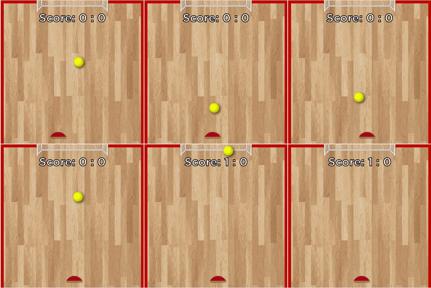
<p>
<img class="postimage_50" src="https://media.giphy.com/media/LhC4oRHFahkxvryfQA/giphy.gif" style="width:40%" />
<figcaption>
<b>Figure 1</b>: This is a popular coding game offered by Code.org. A student would write a program to create this game.
</figcaption>
</p>

<p>Programming a game that is playable is exciting for students who are learning to code. <a href="https://code.org">Code.org</a> provides many game development assignments in their curriculum. In these assignments, students write JavaScript programs in a code editor embedded in the web browser. Game assignments are great for teachers to examine student’s progress as well: students not only need to grasp basic concepts like if-conditionals and for-loops but use these concepts to write the physical rules of the game world — calculate the trajectories of objects, resolve inelastic collision of two objects, and keep track of game states. To deal with all of these complexities, students need to use abstraction (functions/class) to encapsulate each functionality in order to manage this complex set of logic.</p>

<p>
<img class="postimage_75" src="/images/2022-03-28-play-to-grade/figure2.png" style="padding:0;" />
<figcaption>
<b>Figure 2</b>: In Code.org, students program in an interactive code interface, where they can write the program in the coding area, hit run and play their game.
</figcaption>
</p>

<p>Automated grading on the code text alone can be an incredibly hard challenge, even for introductory level computer science assignments. As examples, two solutions which are only slightly different in text can have very different behaviors, and two solutions that are written in very different ways can have the same behaviors. As such, some models that people develop for grading code can be as complex as those used to understand paragraphs of natural language. But, sometimes, grading code can be even more difficult than grading an essay because coding submissions can be in different programming languages. In this situation, one must not only develop a program that can understand many programming languages, but guard against the potential that the grader is more accurate for some languages than others. A Finally, these programs must be able to generalize to new assignments because correct grading is just as necessary for the first student working on an assignment as the millionth – the collect-data, train, deploy cycle is not quite suitable in this context. We don’t have the luxury of collecting a massive amount of labeled dataset to train a fully supervised learning algorithm for each and every assignment.</p>

<p>In a <a href="https://arxiv.org/abs/2110.14615">recent paper</a>, we circumvent these challenges by developing a method that grades assignments by playing them, without needing to look at the source code at all. Despite this different approach, our method still manages to provide scalable feedback that potentially can be deployed in a massively-online setting.</p>

<h2 id="the-play-to-grade-challenge">The Play to Grade Challenge</h2>

<p>Our solution to these problems is to ignore the code text entirely and to grade an assignment by having a grading algorithm play it. We represent the underlying game of each program submission as a Markov Decision Process (MDP), which defines a state space, action space, reward function, and transition dynamics. By running each student’s program, we can build the MDP directly without needing to read or understand the underlying code. You can read more about the MDP framework here: <sup id="fnref:lilianweng" role="doc-noteref"><a href="#fn:lilianweng" class="footnote" rel="footnote">3</a></sup>.</p>

<p>Since all student programs are written for the same assignment, these programs should generate MDP with a lot of commonalities, such as shared state and action space. After playing the game and fully constructing the MDP for an assignment, all we need is to compare the MDP specified by the student’s program (student MDP) to the teacher’s solution (reference MDP) and determine <strong>if these two MDPs are the same</strong>. What sets this challenge apart from any other reinforcement learning problems is the fact that a <strong>classification</strong> needs to be made at the end of this agent’s interaction with this MDP — the decision of whether the MDP is the same as the reference MDP or not.</p>

<p>
<img class="postfigurethird" src="/images/2022-03-28-play-to-grade/distance.png" style="padding:0;" />
<figcaption>
<b>Figure 3</b>: We need to build an approximate distance function D that determines the distance between the student program's underlying MDP (black dot) and correct MDPs (blue dots) and incorrect MDPs (red dots). Read more about how we build this distance function in our <a href="https://arxiv.org/abs/2110.14615">paper</a>.
</figcaption>
</p>

<p>In order to solve this challenge, we present an algorithm with two components: an agent that plays the game and can reliably reach bug states, and a classifier that can recognize bug states (i.e., provide the probability of the observed state being a bug). Both components are necessary for accurate grading: an agent that reaches all states but cannot determine if any represents bugs is just as bad as a perfect classifier paired with an agent that is bad at taking actions which might cause bugs. Imagine a non-optimal agent that never catches the ball (in the example above) – this agent will never be able to test if the wall, or paddle, or goal does not behave correctly.</p>

<p>An ideal agent needs to produce <strong>differential trajectories</strong>, i.e., sequences of actions that can be used to differentiate two MDPs, and must contain at least one bug-triggering state if the trajectory is produced from the incorrect MDP. Therefore, we need both a correct MDP and a few incorrect MDPs to teach the agent and the classifier. These incorrect MDPs are incorrect solutions that can either be provided by the teacher, or come from manually grading a few student programs to find common issues. Although having to manually label incorrect MDPs is an annoyance, we show that the total amount of effort is generally significantly lower than grading each assignment: in fact, we show that for the task we solve in the paper, you only need 5 incorrect MDPs to reach a decent performance (see the appendix section of our paper).</p>

<p>
<img class="postimage_75" src="/images/2022-03-28-play-to-grade/figure3_new.png" style="padding:0;" />
<figcaption>
<b>Figure 4</b>: We build an MDP wrapper around the student program that allows the agent to interact with the program (while the original program might only allow human control, i.e., we override mouse / keyboard events.
</figcaption>
</p>

<h2 id="recognizing-bugs-from-scratch">Recognizing Bugs from Scratch</h2>

<p>Here are three incorrect programs and what they look like when played. Each incorrect program behaves differently from the correct program:</p>
<ul>
  <li>One program’s wall does not allow the ball to bounce on it.</li>
  <li>Another program’s goal post does not let the ball go through.</li>
  <li>The last program spawns 2 new balls whenever the ball bounces on the wall.</li>
</ul>

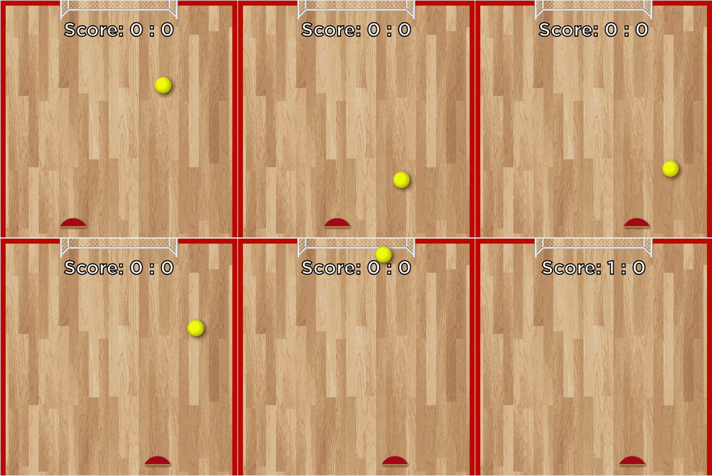
<p><img class="postfigurethird" src="https://media.giphy.com/media/i8ITbB6QtNS67t9dk6/giphy.gif" /> <img class="postfigurethird" src="https://media.giphy.com/media/JuQn32VatSaW1vFCgi/giphy.gif" /><img class="postfigurethird" src="https://media.giphy.com/media/gQKLJuq49sjjkEube9/giphy.gif" /></p>
<figcaption><b>Figure 5</b>: Different types of incorrect student programs.
</figcaption>

<p>A challenge with building differential trajectories is that one must know which state is a bug triggering state. Previous works <sup id="fnref:3" role="doc-noteref"><a href="#fn:3" class="footnote" rel="footnote">4</a></sup><sup id="fnref:4" role="doc-noteref"><a href="#fn:4" class="footnote" rel="footnote">5</a></sup><sup id="fnref:5" role="doc-noteref"><a href="#fn:5" class="footnote" rel="footnote">6</a></sup> have made the strong assumption that one would automatically know when they encountered a bug, potentially because they expect the game program to crash after encountering a bug. Because of this assumption, they focus their efforts on building pure-exploration agents that try to visit as many states as possible. However, in reality, bugs can be difficult to identify and do not all cause the game to crash. For example, a ball that is supposed to bounce off of a wall is now piercing through it and flying off into oblivion. These types of behavioral anomalies motivate the use of a predictive model that can take in the current game state and determine whether it is anomalous or not.</p>

<p>
<img class="postimage_75" src="/images/2022-03-28-play-to-grade/figure4.png" style="padding:0;" />
<figcaption>
<b>Figure 6</b>: The chicken-and-egg cold-start problem. The agent doesn't know how to reach bug state, and the classifier does not know what is a bug.
</figcaption>
</p>

<p>Unfortunately, training a model to predict if a state is a bug state is non-trivial. This is because, although we have labels for some MDPs, these labels are not on the state-level (i.e., not all states in an incorrect MDP are bug states). Put another way, our labels can tell us when a bug has been encountered but cannot tell us what specific action caused the bug. The determination of whether bugs exist in a program can be framed as a chicken-and-egg problem where, if bug states could be unambiguously determined one would only need to explore the state space, and if the exploration was optimal one would only need to figure out how to determine if the current state exhibited a bug.</p>

<h2 id="collaborative-reinforcement-learning">Collaborative Reinforcement Learning</h2>

<p>Fortunately, these types of problems can generally be solved through the expectation-maximization framework, which involves an intimate collaboration between the neural network classifier and the reinforcement learning agent. We propose <strong>collaborative reinforcement learning</strong>, an expectation-maximization approach, where we use a random agent to produce a dataset of trajectories from the correct and incorrect MDP to teach the classifier. Then the classifier would assign a score to each state indicating how much the classifier believes the state is a bug-triggering state. We use this score as reward and train the agent to reach these states as often as possible for a new dataset of trajectories to train the classifier.</p>

<p>After using the RL agent to interact with the MDP to produce trajectories, we can try out  different ways to learn a classifier that can classify a state as a bug or not (a binary label). Choosing the right label  is important because this label will become the reward function for the agent, so it can learn to reach bug states more efficiently. However, we only know if the MDP (the submitted code) is correct or broken, but we don’t have labels for the underlying states. Learning state-level labels becomes a challenge!</p>

<p>We tested out several types of classifiers: (1) a noisy classifier that classifies all states in a broken MDP as broken, (2) a Gaussian Mixture Model that treats all states independently, (3) a Variational Autoencoder that also treats all states independently but directly models non-linear interactions among the features, or (4) an LSTM that jointly models the teacher program as an MDP (HoareLSTM) and an LSTM that models the student program as an MDP (Contrastive HoareLSTM) – with a distance function that compares the two MDPs, borrowing distance notions from literature in MDP homomorphism<sup id="fnref:homomorph" role="doc-noteref"><a href="#fn:homomorph" class="footnote" rel="footnote">7</a></sup><sup id="fnref:lihong" role="doc-noteref"><a href="#fn:lihong" class="footnote" rel="footnote">8</a></sup><sup id="fnref:kipf" role="doc-noteref"><a href="#fn:kipf" class="footnote" rel="footnote">9</a></sup><sup id="fnref:givan" role="doc-noteref"><a href="#fn:givan" class="footnote" rel="footnote">10</a></sup>.</p>

<p>In this toy environment, the agent drives a car on a 2D plane. Whenever the agent drives the car into the outer rim of this area (space between the boundary and red dotted line), a bug will cause the car to get stuck (Leftmost panel in <a href="#figure5">Figure 5</a>). Being stuck means the car’s physical movement is altered, resulting in back-and-forth movement around the same location. The bug classifier needs to recognize the resulting states (position and velocity) of the car being “stuck”, by correctly outputting a binary label (bug) for these states.</p>

<p>In this setting, there is only one type of bug. Most classifiers do well when the agent only drives a straight line (single-direction agent). However, when the agent randomly samples actions at each state, simpler classifiers can no longer differentiate between bug and non-bug states with high accuracy.</p>

<p>
<a id="figure5"></a>
<img class="postfigurethird" src="/images/2022-03-28-play-to-grade/figure5_env.png" style="padding:0; width:25%" />
<img class="postfigurethird" src="/images/2022-03-28-play-to-grade/figure5_single_direction_agent.png" style="padding:0; width:35%" />
<img class="postfigurethird" src="/images/2022-03-28-play-to-grade/figure5_random_agent.png" style="padding:0;width:35%" />
<figcaption>
<b>Figure 7</b>: Performance of different bug classification models with different RL agents.
</figcaption>
</p>

<p>We can increase the difficulty of this setting to see if collaborative training can make the agent operate in the environment with an intention to trigger bugs. In this toy environment, now the bugs will only be triggered in red boxes (Leftmost panel in <a href="#figure6">Figure 6</a> below). We can see that with only one round of collaborative training (“CT Round 1”), the performances of ALL classifiers are improved, including weaker classifiers. This is understandable, as the agent learns to gradually collect better datasets to train classifiers – and higher quality datasets lead to stronger classifiers. For example, variational auto-encoder started only with 32% precision, but it increased to 74.8% precision after 2 rounds of collaborative training.</p>

<p>
<a id="figure6"></a>
<img class="postfigurethird" src="/images/2022-03-28-play-to-grade/figure6_env.png" style="padding:0; width:25%" />
<img class="postfigurethird" src="/images/2022-03-28-play-to-grade/figure6_training_improvement_with_CI.png" style="padding:0; width:70%" />
<figcaption>
<b>Figure 8</b>: Collaborative training improves bug classifier performance across different models. This shows how important it is for the RL agent to produce <b>differential trajectories</b>, which will allow classifiers to obtain higher performance.
</figcaption>
</p>

<p>We can also visualize how the collaborative training quickly allows the agent to learn to explore states that most-likely contain bugs by visualizing the trajectories (see figure below). Initially the agent just explores the space uniformly (blue curves), but after one round of collaborative training (CT), it learns to focus on visiting the potential bug areas (regions marked by red boxes) (red curves).</p>

<p><a id="figure7"></a><br />
<img class="postimage_75" src="/images/2022-03-28-play-to-grade/figure7.png" style="padding:0;" /></p>
<figcaption>
<b>Figure 9</b>: Visualization of the paths taken by the RL agent (each line represents one trajectory). After collaborative training (CT), the agent quickly focuses only on visiting potentially bug states (relying on the signal provided by the bug classifiers).
</figcaption>

<h2 id="grading-bounce">Grading Bounce</h2>

<p>Next, we returned to the motivating example for this type of approach: grading real student submissions. With help from <a href="https://code.org">Code.org</a>, we are able to verify the algorithm’s performance on a massive amount of unlabeled, ungraded student submissions. The game <a href="https://studio.code.org/s/course3/lessons/15/levels/10">Bounce</a>, from Code.org’s <a href="https://studio.code.org/s/course3/">Course3</a> for students in 4th and 5th grade, provides a real-life dataset of what variations of different bugs and behaviors in student programs should look like. The dataset is compiled of 453,211 students who made an attempt on this assignment. In total, this dataset consists of 711,274 programs.</p>

<p><a id="figure8"></a><br />
<img class="postimage_50" src="/images/2022-03-28-play-to-grade/figure8_table.png" style="padding:0;" /></p>
<figcaption>
<b>Figure 10</b>: Each program has a binary label (correct or broken) associated with it. We only have 11 programs as our training data.
</figcaption>

<p>We train our agent and classifier on 10 broken programs that we wrote without looking at any of the student’s submissions. The 10 programs contain bugs that we “guess” to be most likely to occur, and we use them to train 10 agents that learn to reach bug states in these 10 programs. This means that in our training dataset, we have 1 correct program and 10 broken programs. Even with only 11 labeled programs, our agent and classifier can get <strong>99.5%</strong> precision at identifying a bug program and <strong>93.4-94%</strong> accuracy overall – the agent is able to trigger most of the bugs and the classifier recognizes the bug states using only 10 broken programs. Though for other games, especially more complicated games, the number of training programs will vary. We strongly believe the number is still in magnitude smaller than training supervised code-as-text algorithms. This demonstration shows the promise of reformulating code assignment grading as the Play to Grade.</p>

<p><a id="figure9"></a><br />
<img class="postimage_75" src="/images/2022-03-28-play-to-grade/figure9_table.png" style="padding:0;" /></p>
<figcaption>
<b>Figure 11</b>: We show superior performance compared to training a simple code-as-text classifier. <b>For complex, interactive programs, Play to Grade is the most data efficient solution.</b>
</figcaption>

<h2 id="what-is-next">What is Next?</h2>

<p>We started this project by making the argument that sometimes it is far easier to grade a complex coding assignment not by looking at the code text but by playing it. Using Bounce, we demonstrated that in the simple task of identifying if a program has a bug or not (a binary task, nonetheless), we are able to achieve striking accuracy with only 11 labeled programs. We provide a simulator and all of the student’s programs on this <a href="https://github.com/windweller/play-to-grade/">Github repo</a>.</p>

<h3 id="multi-label-bounce">Multi-label Bounce</h3>

<p>One promising direction for future work is to expand beyond pass/fail binary feedback, and actually identify which bug is in the student’s program and provide that information. Our Bounce dataset enables this by providing multi-error labels, as shown in the table below. The multi-error label setting was not solved by our current algorithm and remains an open challenge!</p>

<p><a id="figure10"></a><br />
<img class="postimage_75" src="/images/2022-03-28-play-to-grade/figure10_multi.png" style="padding:0;" /></p>
<figcaption>
<b>Figure 12</b>: Each program has a binary label (correct or broken) associated with it. We only have 11 programs as our training data.
</figcaption>

<h3 id="more-than-one-correct-solution">More than One Correct Solution</h3>

<p>Oftentimes, students create solutions that are creative. Creative solutions are different, but not wrong. For example, students can change the texture pattern of the ball or paddle; or they can make the paddle move much faster. How to set the boundary between “being creative” and “being wrong”? This is not a discussion that happens often in AI, but is of huge importance in education. Though we didn’t use the Bounce dataset to focus on the problem of understanding creativity, our work can still use distance measures to set a “tolerance threshold” to account for creativity.</p>

<h3 id="for-educators">For Educators</h3>

<p>We are interested in collecting a suite of interactive coding assignments and creating a dataset for future researchers to work on this problem. Feel free to reach out to us and let us know what you would consider as important in grading and giving students feedback on their coding assignments!</p>

<h2 id="conclusion">Conclusion</h2>

<p>Providing automated feedback for coding is an important area of research in computational education, and an important area for building fully autonomous coding education pipeline (that can generate coding assignment, grade assignment, and teach interactively). Providing a generalizable algorithm that can play interactive student programs in order to give feedback is an important problem for education and an exciting intellectual challenge for the reinforcement learning community. In this work, we introduce the challenge and a dataset, set up the MDP distance framework that is highly data efficient, algorithms that achieve high accuracy, and demonstrate this is a promising direction of applying machine learning to assist education.</p>

<p>This blog post is based on the following paper:</p>

<ul>
  <li>“Play to Grade: Testing Coding Games as Classifying Markov Decision Process.” Allen Nie, Emma Brunskill, and Chris Piech. Advances in Neural Information Processing Systems 34 (2021).</li>
</ul>

<h2 id="acknowledgements">Acknowledgements</h2>

<p>Many thanks to Emma Brunskill, Chris Piech for their guidance on the project. Many thanks to Mike Wu, Ali Malik, Yunsung Kim, Lisa Yan, Tong Mu, and Henry Zhu for their discussion and feedback. Special thanks to <a href="https://www.code.org">code.org</a>, and Baker Franke, for many years of collaboration and generously providing the research community with data. Thanks to Stanford Hoffman-Yee Human Centered AI grant for supporting AI in education. Thanks for the numerous rounds o edits from Megha Srivastava and Jacob Schreiber.</p>

<div class="footnotes" role="doc-endnotes">
  <ol>
    <li id="fn:codeorgstats" role="doc-endnote">
      <p>Code.org displays this statistics on their landing webpage. <a href="#fnref:codeorgstats" class="reversefootnote" role="doc-backlink">&#8617;</a></p>
    </li>
    <li id="fn:2" role="doc-endnote">
      <p>William G Bowen. The ‘cost disease’ in higher education: is technology the answer? The Tanner Lectures Stanford University, 2012. <a href="#fnref:2" class="reversefootnote" role="doc-backlink">&#8617;</a></p>
    </li>
    <li id="fn:lilianweng" role="doc-endnote">
      <p><a href="https://lilianweng.github.io/lil-log/2018/02/19/a-long-peek-into-reinforcement-learning.html">https://lilianweng.github.io/lil-log/2018/02/19/a-long-peek-into-reinforcement-learning.html</a> <a href="#fnref:lilianweng" class="reversefootnote" role="doc-backlink">&#8617;</a></p>
    </li>
    <li id="fn:3" role="doc-endnote">
      <p>Gordillo, Camilo, Joakim Bergdahl, Konrad Tollmar, and Linus Gisslén. “Improving Playtesting Coverage via Curiosity Driven Reinforcement Learning Agents.” arXiv preprint arXiv:2103.13798 (2021). <a href="#fnref:3" class="reversefootnote" role="doc-backlink">&#8617;</a></p>
    </li>
    <li id="fn:4" role="doc-endnote">
      <p>Zhan, Zeping, Batu Aytemiz, and Adam M. Smith. “Taking the scenic route: Automatic exploration for videogames.” arXiv preprint arXiv:1812.03125 (2018). <a href="#fnref:4" class="reversefootnote" role="doc-backlink">&#8617;</a></p>
    </li>
    <li id="fn:5" role="doc-endnote">
      <p>Zheng, Yan, Xiaofei Xie, Ting Su, Lei Ma, Jianye Hao, Zhaopeng Meng, Yang Liu, Ruimin Shen, Yingfeng Chen, and Changjie Fan. “Wuji: Automatic online combat game testing using evolutionary deep reinforcement learning.” In 2019 34th IEEE/ACM International Conference on Automated Software Engineering (ASE), pp. 772-784. IEEE, 2019. <a href="#fnref:5" class="reversefootnote" role="doc-backlink">&#8617;</a></p>
    </li>
    <li id="fn:homomorph" role="doc-endnote">
      <p>Pablo Samuel Castro, Prakash Panangaden, and Doina Precup. Equivalence relations in fully and partially observable markov decision processes. In Twenty-First International Joint Conference on Artificial Intelligence, 2009. <a href="#fnref:homomorph" class="reversefootnote" role="doc-backlink">&#8617;</a></p>
    </li>
    <li id="fn:lihong" role="doc-endnote">
      <p>Lihong Li, Thomas J Walsh, and Michael L Littman. Towards a unified theory of state abstraction for mdps. ISAIM, 4:5, 2006. <a href="#fnref:lihong" class="reversefootnote" role="doc-backlink">&#8617;</a></p>
    </li>
    <li id="fn:kipf" role="doc-endnote">
      <p>Elise van der Pol, Thomas Kipf, Frans A Oliehoek, and Max Welling. Plannable approximations to mdp homomorphisms: Equivariance under actions. arXiv preprint arXiv:2002.11963, 2020. <a href="#fnref:kipf" class="reversefootnote" role="doc-backlink">&#8617;</a></p>
    </li>
    <li id="fn:givan" role="doc-endnote">
      <p>Robert Givan, Thomas Dean, and Matthew Greig. Equivalence notions and model minimization in markov decision processes. Artificial Intelligence, 147(1-2):163–223, 2003. <a href="#fnref:givan" class="reversefootnote" role="doc-backlink">&#8617;</a></p>
    </li>
  </ol>
</div>]]></content><author><name></name></author><summary type="html"><![CDATA[[Summary] tl;dr: A tremendous amount of effort has been poured into training AI algorithms to competitively play games that computers have traditionally had trouble with, such as the retro games published by Atari, Go, DotA, and StarCraft II. The practical machine learning knowledge accumulated in developing these algorithms has paved the way for people to now routinely train game-playing AI agents for many games. Following this line of work, we focus on a specific category of games – those developed by students as part of a programming assignment. Can the same algorithms that master Atari games help us grade these game assignments? In our recent NeurIPS 2021 paper, we illustrate the challenges in treating interactive coding assignment grading as game playing and introduce the Play to Grade Challenge.]]></summary></entry><entry><title type="html">Rational Speech Act For Controllable Image Caption Generation</title><link href="https://anie.me/vqa-caption/" rel="alternate" type="text/html" title="Rational Speech Act For Controllable Image Caption Generation" /><published>2020-05-06T00:00:00+00:00</published><updated>2020-05-06T00:00:00+00:00</updated><id>https://anie.me/vqa-caption</id><content type="html" xml:base="https://anie.me/vqa-caption/"><![CDATA[<p><a href="https://arxiv.org/abs/2004.14451">[Paper]</a></p>

<p>In the past two years, controlling generative models (such as GANs and VAEs) have been widely studied in the Computer Vision literature. The idea is that once these large capacity neural network models learn the data manifold of millions of images, it has internalized some knowledge about the world. The “knowledge” learned is often in the form of abstract concepts such as “skin tone”, “hair style” from faces, or “brightness”, “rotation angles” for general images. We can then explicitly control images generated from GAN or VAE with respect to these abstract concepts through some post-training manipulations.</p>

<p style="text-align: center"><img src="https://github.com/allenanie/allenanie.github.io/blob/master/images/bayesian_decoding/RSA_GAN_VAE.png?raw=true" style="width:120%" /> <br /> <span>Figure 1: (a) from OpenAI GLOW demo; (b) from ICLR 2020 paper: On the "steerability" of generative adversarial networks.</span> </p>

<p>Despite such an impressive result, controlling generative models in text has been far more difficult. Limited successes have been achieved for properties like sentiment or tense (Hu et al.<sup id="fnref:1" role="doc-noteref"><a href="#fn:1" class="footnote" rel="footnote">1</a></sup>). Further work from Lample et al.<sup id="fnref:2" role="doc-noteref"><a href="#fn:2" class="footnote" rel="footnote">2</a></sup> leveraged the domain where the data are collected to add additional attributes such as gender, race, age, and interests (like music, book, movie, etc.), and trained a neural network from scratch conditioned on these attributes. However, for vagueness, politeness, genericness, sarcasm, humor, and formality, we have made little progress in developing neural network based decoding method to control these aspects of text.</p>

<p>In this post, we will focus on one: Question-under-Discussion (QuD). When we communicate with each other, there is often an implicit question under discussion (hence the name). For example, when two strangers meet, the QuD would often be “tell something about yourself”, so people often start with self-introduction. However, instead of listing all the facts about oneself (starting from age, height), people usually choose to communicate more relvant facts about themselves given the situation. In a blind date, people talk about their interests, income, attitudes towards starting a family, dating preferences etc. In a business metting, people talk about their professional history.</p>

<p>The QuD model has been formalized in 1984 as a model of discourse. It emphasizes on the fact that we communicate the state of the world <strong>up to a partition</strong>. The partition often refers to context (or in this case, the QuD that specifies the context).</p>

<p>As a general discourse model, QuD model goes beyond simple conversation. It suggests that for every sentence we say or write, there is a corresponding underlying question; even for paragraphs of text that we write. QuD Model turns any paragraph of text into a self-conversation in a writer’s head.</p>

<p>Here is an example, if I start with the sentence “A few of us arrive at the classroom and the door is locked.” What should I write next? As you can see, QuD dictates how I write my next sentence. QuD decides what’s relevant in this situation and what’s not.</p>

<table>
  <thead>
    <tr>
      <th>QuD</th>
      <th>Paragraph (next sentence in bold)</th>
    </tr>
  </thead>
  <tbody>
    <tr>
      <td>Why is the room locked?</td>
      <td>A few of us arrive at the classroom and the door is locked. <strong>We realize the teacher has not arrived.</strong></td>
    </tr>
    <tr>
      <td>Who has the key?</td>
      <td>A few of us arrive at the classroom and the door is locked. <strong>None of us has the key.</strong></td>
    </tr>
    <tr>
      <td>Does Stefanie have the key?</td>
      <td>A few of us arrive at the classroom and the door is locked. <strong>Stefanie does not have the key.</strong></td>
    </tr>
    <tr>
      <td>Is there another class in the room?</td>
      <td>A few of us arrive at the classroom and the door is locked. <strong>Through the window, the room appears to be empty.</strong></td>
    </tr>
  </tbody>
</table>

<p>Even though all of my next sentences are direct followup of the previous sentence (often referred to as “context” or “scenario”), they are all quite different because I’m addressing different QuDs. In another word, if our generative model for text is QuD-sensitive, we can control text generation by swapping QuDs.</p>

<p>Maybe you can already see what we want to do: an image can serve as scenario/context, questions from VQA (Visual Question Answering dataset) can serve as QuDs , and sentence generated by the image captioner are the “next sentence” we want to generate. By changing the question, our method will change the generated caption. Cool, huh? There is no attribute classifier, no additional annotated training data,  just a question and an image.</p>

<p>If we are able to achive this – using a QuD (natural language question) to ask the model to focus on different features of the image, we open the door to truly flexible controllable text generation. For the same image, I can ask: “Can the man run far?”, and the caption can be “This is a runner who jogs through the entire park.” Or I can ask “Does this man look tired?”, and the caption can be “The man is energetically running.”</p>

<p>So the idea seems fun, but is this technologically possible? Remember, there is no additional training involved. How can an image captioner that is only trained on image caption dataset be sensitive to questions from a VQA dataset? To answer this question, we need to rethink what question is and introduce Rational Speech Act (RSA)  framework. A more technical overview of this is described in my new paper with with Reuben Cohn-Gordon and Chris Potts<sup id="fnref:6" role="doc-noteref"><a href="#fn:6" class="footnote" rel="footnote">3</a></sup>.</p>

<h2 id="qud-in-image-captioning">QuD in Image Captioning</h2>

<p style="text-align: center"><img src="https://github.com/allenanie/allenanie.github.io/blob/master/images/bayesian_decoding/fig5_large.png?raw=true" style="width:120%" /> <br /> <span>Figure 2: Examples from applying our method to a SoTA 6-layer encoder-decoder Transformer with 55M parameters image captioner trained on the MS COCO dataset. The base caption shows what the Transformer originally would have outputted(last column). The penultimate column (Issue-sensitive caption) shows what our method would produce. We can produce captions that try to address a question.</span> </p>

<p>VQA style questions focus on three things: object, attribute of the object, relationship between objects. If we think more carefully about a useful representation of an image (let’s say if we want an image to someone who can’t see), we will describe the first picture in Figure 2 as “There’s grass on the ground. The photo is captured through a net. There is a guy wearing orange jersey, white pants, and he’s throwing a baseball. This guy is a pitcher. He’s standing on a field”. We can write this more structurally into a list, where we would list every object, its every attribute (color, weight, texture, etc.), and its relationship to other object in the picture. Needless to say, this list will be incredibly long and I personally doubt if it can ever be “complete”.</p>

<p>This is how we write down captions for each image – we write down a small amount of features in the image that catch our attention. That is to say: human captions attempt to address an indeterminate question (or “all” questions). The captioning system learns to map features in an image to a grammatical sequence of words. To change the caption with respect to a question, what we mean is that we want the caption to reflect a particular feature the question is seeking. If the question is “What position is this man playing?”, then the caption needs to mention a feature which is this guy’s position (i.e., “pitcher”). We call this Issue-Sensitive Image Captioning (ISIC) because we want the generated caption to resolve an issue (question).</p>

<p>We show some preliminary success in Figure 2. By asking questions such as “what color is the sky”, we control the image captioner to focus on a particular nature of this photo (that this is a black &amp; white photo). Instead of describing what is the scene of the picture (“airplane taking off”), the caption model describes the meta-level information of this picture: (“a black and white photo of an airplane”).</p>

<p>Examining controllable text generation in a multi-modal domain (image, text) allows us to clearly define the question (through a pre-collected VQA dataset). Since image datasets are often densely annotated (with object information, attributes of objects, etc.), we can automatically evaluate whether our generated caption addresses the question (from here on, we refer to this as “resolve the issue”). However, even with dense annotations, evaluating issue resolution is still a major challenge. We evaluate our proposed method on a restricted domain of bird images (CUB-2011), but we showed some promising examples in a more general dataset such as MSCOCO (in Figure 2).</p>

<h2 id="controlling-via-rsa-a-simple-tour">Controlling via RSA: A Simple Tour</h2>

<p>In the previous section, we have established that in order to be question-aware, captions need to describe a feature in the image that is the answer to the question. Then we can think of the process to make our model generate question-aware captions as the process of picking out the right features that will answer the question. This is when RSA comes in.</p>

<p>The Rational Speech Act (RSA) is a framework of Bayesian models for cognition and language. It turns out a simple model in this family is highly revelant for machine learning tasks, since it captures the idea of referential language generation (which I will describe below). Computing this model turns out to require only simple matrix operations, which is extremely suitable and modular to apply to any large neural network model.</p>

<p style="text-align: center"><img src="https://github.com/allenanie/allenanie.github.io/blob/master/images/bayesian_decoding/police_lineup.jpg?raw=true" style="width:70%" /> <br /> <span>Source: New Yorker; University of Michigan, Law School. </span> </p>

<p>Here’s the intuition on what human thought process RSA is trying to capture. If you were asked to say a word to the police so that they can pick out number 5 (but you are not allowed to say numbers), you probably would not say “a man,” nor would you say “khaki pants”. The best word you can pick (assuming you are rational) is “baseball cap” because it uniquely identifies number 5. RSA is created to emulate this thought process – when you have a group of images, you want to pick the word that best represents it (so that it’s distinguishing the target image from the rest).</p>

<p>The computational process for the simplest RSA model can be easily achieved through Bayes rule – probability matrix normalization. In this formulation, a simplified version of our pre-trained image captioner model is $S_0(\mathbf{w} \vert \mathbf{i})$, a row-stochastic probability matrix (probabilities in a row sum up to 1) where the rows are “images”, represented as a list of features, and the columns are the features we can pick to represent the image. How is this a captioning model? Well, you can imagine a captioning model that only produces one word (represented as an emoji in our schema).</p>

<p style="text-align: center"><img src="https://github.com/allenanie/allenanie.github.io/blob/master/images/bayesian_decoding/RSA_simple.png?raw=true" style="width:100%" /> <br /> <span>Figure 3: A simple RSA computing process. </span> </p>

<p>Without considering the goal of contrasting two other images, for the first image, we will choose either  <code class="language-plaintext highlighter-rouge">baseball cap</code> or <code class="language-plaintext highlighter-rouge">mountain</code> to describe it. However, if we want to uniquely identify this image (to a police officer, or to anyone who’s “listening”) against the other two images, we would realize that the other two rows also have mountains. What’s unique about the first row is the <code class="language-plaintext highlighter-rouge">baseball cap</code>.</p>

<p>The process described in Figure 3 is extremely simple but captures the process of reasoning about  plausible alternatives and then decide what to select to achieve its best unambiguous outcome. We can see in bold number that $S_1$ will choose <code class="language-plaintext highlighter-rouge">baseball cap</code> to describe the first image, contrasting the other two.</p>

<p>More formally, these two computations can be described as:</p>

<pre>\begin{align*}
L_1(\mathbf{i}|\mathbf{w}) &amp;= \frac{S_0(\mathbf{w}|\mathbf{i}) P(\mathbf{i})}{P(\mathbf{w})} = \frac{S_0(\mathbf{w}|\mathbf{i}) P(\mathbf{i})}{\sum_{i \in \mathcal{I}} S_0(\mathbf{w}|\mathbf{i}) P(\mathbf{i})} \\
S_1(\mathbf{w}|\mathbf{i}) &amp;= \frac{L_1(\mathbf{i}|\mathbf{w}) P(\mathbf{w})}{P(\mathbf{i})} = \frac{L_1(\mathbf{i}|\mathbf{w}) P(\mathbf{w})}{\sum_{w \in \mathcal{V}} L_1(\mathbf{i}|\mathbf{w}) P(\mathbf{w})} \\
\end{align*}</pre>

<p>In RSA books/papers, you often see the simplified version (skipping the normalization constant):</p>

<pre>\begin{align*}
L_1(\mathbf{i}\vert\mathbf{w}) &amp;\propto S_0(\mathbf{w}|\mathbf{i}) P(\mathbf{i}) \\
S_1(\mathbf{w}\vert\mathbf{i}) &amp;\propto L_1(\mathbf{i}|\mathbf{w})P(\mathbf{w})
\end{align*}</pre>

<p>More detailed tutorial of RSA can be found in <a href="https://www.problang.org/">here</a>.</p>

<h2 id="rsa--vqa-is-our-caption-question-aware">RSA + VQA: Is Our Caption Question-Aware?</h2>

<p>Equipped with the knowledge of RSA, in order to achieve our goal, all we need to do is to pick out a set of images so that for the target image, the caption we produce will contain the feature that is the answer to the question. We will now describe a procedure to select a set of images so that our caption model and our RSA re-weighting will put high probability on features that can answer our question.</p>

<p>Given a target image and a question: $(\mathbf{i}, \mathbf{q})$, we can directly apply any pre-trained VQA model to get an answer. Given a lot of images and the same question, we can get a lot of answers. Some of these answers are different from the answer for the target image, some are the same. For example, with our target image: <code class="language-plaintext highlighter-rouge">{blue baseball cap, mountain}</code>, we can ask the following  question: <code class="language-plaintext highlighter-rouge">Does the person wear a baseball cap?</code>, where the answer is <code class="language-plaintext highlighter-rouge">Yes</code> or <code class="language-plaintext highlighter-rouge">No</code>.</p>

<p>Given this answer, we can partition a list of images into two groups: images where the person is wearing a baseball cap, and images where the person is NOT wearing a baseball cap. Note that the question can be extremely general and ask about various aspects of the image.</p>

<p>Suppose we happen to select these 6 images from a larger group of images. First three images have baseball cap, the next three do not. Can we just naively apply RSA and hope the item we pick will be about the baseball cap? The answer is unfortunately no. Before RSA, the caption model will randomly choose between baseball cap and mountain. After RSA, it will choose mountain, which is worse.</p>

<p style="text-align: center"><img src="https://github.com/allenanie/allenanie.github.io/blob/master/images/bayesian_decoding/RSA_comp_fig.png?raw=true" style="width:100%" /> <br /> <span>Figure 5: Directly applying RSA is NOT question-aware (or issue-sensitive, as defined in our paper).</span> </p>

<p>OK. We ran into a problem: even though our VQA model <strong>partitioned 6 images into two cells</strong> (top 3 rows and bottom 3 rows), the RSA computation is unaware of this (cell structure). What it does is treating all 5 other images (rows) as distractors and try to find what’s unique about the target image (first row) against all else, which is the mountain.</p>

<p>Luckily, a solution has already been worked out by Kao et al. <sup id="fnref:7" role="doc-noteref"><a href="#fn:7" class="footnote" rel="footnote">4</a></sup> The idea is pretty simple, why not just add up the probability within the cell (across the column) after computing $L_1$ probability matrix? More formally, this corresponds a different $S_1$:</p>

<pre>
\begin{align*}
U_1^{\mathbf{C}}(\mathbf{i}, \mathbf{w}, \mathbf{C}) &amp;= \log \Big( \sum_{\mathbf{i}' \in \mathcal{I}}\delta_{\mathbf{C}(\mathbf{i})=\mathbf{C}(\mathbf{i}')} L_1(\mathbf{i}'|\mathbf{w}) \Big) \\
S_1^{\mathbf{C}}(\mathbf{w} \vert \mathbf{i}, \mathbf{C}) &amp;\propto \text{exp} \big(\alpha U_1^{\mathbf{C}}(\mathbf{i}, \mathbf{w}, \mathbf{C}) - \text{cost}(\mathbf{w}) \big)
\end{align*}
</pre>

<p>This formula redefines the pragmatic listener matrix $L_1$ as an informative utility $U_1^{\mathbf{C}}$, and compute $S_1$ probability matrix proportional to it. In the RSA literature, this is often referred to as the QuD-RSA (QuD: Question-under-Discussion). If we visualize this process with actual probability numbers, here’s the result:</p>

<p style="text-align: center"><img src="https://github.com/allenanie/allenanie.github.io/blob/master/images/bayesian_decoding/RSA_Q_U1.png?raw=true" style="width:70%" /> <br /> <span>Figure 6: We show the computational process of QuD-RSA.</span> </p>

<p>As you can see, what we really did is just add up along the column for the original $L_1$ matrix, and then normalize over the row for the target image. This allows our RSA output to be issue-sensitive (question-aware). But wait wait wait, something is not right here! If you actually looked very closely at the $S_1^\mathbf{C}$ table, you’d realize what the RSA picked out is still wrong – it would randomly choose between <code class="language-plaintext highlighter-rouge">skiing</code> and <code class="language-plaintext highlighter-rouge">mountain</code>. What the heck is going on?</p>

<p>So, what QuD-RSA actually does is that, it creates an “equivalence class” between all images in the same cell. It converts the original objective, which is to “pick an item to best describe target image” to “pick an item to best describe the target cell”. QuD-RSA is designed to ignore the differences between within-cell images. Since picking <code class="language-plaintext highlighter-rouge">mountain</code> or <code class="language-plaintext highlighter-rouge">skiing</code> (neither appeared in the distractor images) would already best identify the target cell, there is no additional incentive to pick <code class="language-plaintext highlighter-rouge">baseball cap</code>. Suffice to say this is not what we want.</p>

<p>This last ingredient allows us to add a pressure to $S_1$ to select items that are shared amongst all images within the cell. Intuitively, since all images within the target cell share the same answer to the VQA question, whatever attribute/object in the image allows that answer will have a higher chance to appear in the resulting caption. This ingredient we choose to add is called <a href="https://en.wikipedia.org/wiki/Entropy_(information_theory)">information entropy</a>, where flatter distribution (more uniformly distributed) will have a higher entropy, and peakier distribution will have a lower entropy. Since <code class="language-plaintext highlighter-rouge">baseball cap</code> is shared among all three images in the target cell, it will have the highest entropy.</p>

<p>More formally, we can write it out to combine both $U_1$ and $U_2$, with a balancing hyper-parameter $\beta \in [0, 1]$ that decides between how much weight we want to put on either utility:</p>

<pre>
\begin{align*}
U_2(\mathbf{i}, \mathbf{w}, \mathbf{C}) &amp;= H(L_1(\mathbf{i}'|\mathbf{w}) \cdot \delta_{\mathbf{C}(\mathbf{i})=\mathbf{C}(\mathbf{i}')}) \\
S_1^{\mathbf{C}+H}(\mathbf{w} \vert \mathbf{i}, \mathbf{C}) &amp;\propto \text{exp} \big( \alpha ((1-\beta)U_1 + \beta U_2) -\text{cost}(\mathbf{w}) \big)
\end{align*}
</pre>

<p>And computationally it can be visualized as:</p>

<p style="text-align: center"><img src="https://github.com/allenanie/allenanie.github.io/blob/master/images/bayesian_decoding/RSA_QH.png?raw=true" style="width:70%" /> <br /> <span>Figure 6: We show the computational process of QuD-Entropy-RSA.</span> </p>

<p>Now the story for generating issue-sensitive (question-aware) captions is complete. With the added entropy reward, the $S_1$ matrix will finally pick <code class="language-plaintext highlighter-rouge">baseball cap</code> as the answer to <code class="language-plaintext highlighter-rouge">What is the person wearing?</code>.</p>

<p>We apply this RSA re-weighting process to every decoder step, which is called Incremental RSA, described in <sup id="fnref:5" role="doc-noteref"><a href="#fn:5" class="footnote" rel="footnote">5</a></sup>. In a seperate blog post, I will share how to write RSA computation as a modular component to add to any image captioning algorithm.</p>

<h2 id="evaluating-on-birds-cub">Evaluating on Birds (CUB)</h2>

<p>Verifying whether we are successful at “controlling” the caption is difficult. We do have a question and an answer in VQA, but how do we determine if the answer is mentioned in the caption? Even for simple attributes like color, for example, “What color is the flower?” with an answer “red”, what captions would satisfy our definition of “addressing the question”?</p>

<blockquote>
  <ol>
    <li>There is a scarlett-colored flower.</li>
    <li>There is a red humming bird flying over a flower.</li>
  </ol>
</blockquote>

<p>The first caption addresses the question (resolves the issue), but the second doesn’t (because “red” is modifying the bird, not the flower). This highlights the type of challenges we need to address for general domain image datasets such as MSCOCO and VQA. So, can we try an automated evaluation for a restricted domain? Turns out, yes.</p>

<p>We use CalTech-UC-San-Diego Bird Dataset (CUB-2011), which has 312 features of birds annotated for each image (11788 images in total), and since it’s a restricted domain, these 312 features are exhaustive for each bird. These features include 26 body parts, such as “belly color”, “bill length”, etc. We can imagine that each body part can be the focus of one question: “What is the belly color of this bird?” and “What is the bill length of this bird”?</p>

<p>We are able to build a simple keyword based classifier that can identify body part mentions in caption as well as attributes (modifiers) of these body parts. We use this classifier to evaluate our method to control caption generation. We refer to this as the “feature-in-text” classifier.</p>

<p>Instead of using VQA, we use the feature matrix annotation as guide to select birds that share similar features (that describe the body parts) with the target image, and birds that don’t share similar features. We show some generated captions below:</p>

<p style="text-align: center"><img src="https://github.com/allenanie/allenanie.github.io/blob/master/images/bayesian_decoding/RSA_bird_ex.png?raw=true" style="width:100%" /> <br /> <span>Figure 7: Generated captions for CUB birds. Left bracket contains images that share the same feature (under discussion) as the target image. Right bracket contains images that don't.</span> </p>

<p>We begin by assessing the extent to which our issues ensitive pragmatic models produce captions that are more richly descriptive of the target image than a base neural captioner. For CUB, we can simply count how many attributes the caption specifies according to our feature-in-text classifier. More precisely, for each image and each model, we generate captions under all resolvable issues, concatenate those captions, and then use the feature-in-text classifier to obtain a list of attributes, which we can then compare to the ground truth for the image as given by the CUB dataset.</p>

<p style="text-align: center"><img src="https://github.com/allenanie/allenanie.github.io/blob/master/images/bayesian_decoding/RSA_table1.png?raw=true" style="width:60%" /> <br /> <span>Table 1</span> </p>

<p>Table 1 reports on this evaluation. Precision for all models is very high; the underlying attributes in CUB are very comprehensive, so all high-quality captioners are likely to do well by this metric. In contrast, the recall scores vary substantially, and they clearly favor the issue-sensitive models, revealing them to be substantially more descriptive than $S_0$.</p>

<p>In Table 2, we provide a breakdown of these scores by body part. The issue-sensitive models are clear winners for all categories. It is noteworthy that the entropy term seems to help for some categories but not others, suggesting underlying variation in the categories themselves. It’s safe to say that some categories are rarely discussed in ground-truth captions thus leading to difficulty for the captioning model to generate them.</p>

<p style="text-align: center"><img src="https://github.com/allenanie/allenanie.github.io/blob/master/images/bayesian_decoding/RSA_table2.png?raw=true" style="width:60%" /> <br /> <span>Table 2</span> </p>

<p>Our previous evaluation shows that varying the issue has a positive effect on the captions generated by our issue-sensitive models, but it does not assess whether these captions resolve individual issues in an intuitive way. We now report on an assessment that quantifies issue-sensitivity in this sense.</p>

<p>The question posed by this method is as follows: for a given issue, does the produced caption precisely resolve the issue? We can divide this into two sub-questions. First, does the caption resolve the issue, which is a notion of recall. Second, does the caption avoid addressing issues that are different from what we want to address, which is a notion of precision. The recall pressure is arguably more important, but the precision one can be seen as assessing how often the caption avoids irrelevant and potentially distracting information.</p>

<p>Overall, the scores reveal that this is a very challenging problem, which traces to the fine-grained issues that CUB supports. Entropy in here proves to be incredibly important to resolve the issue.</p>

<p style="text-align: center"><img src="https://github.com/allenanie/allenanie.github.io/blob/master/images/bayesian_decoding/RSA_table3.png?raw=true" style="width:60%" /> <br /> <span>Table 3</span> </p>

<h2 id="conclusion">Conclusion</h2>

<p>Obviously there are a lot left to be done. We defined the task of Issue-Sensitive Image Captioning (ISIC) and developed a Bayesian pragmatic model that allows us to address this task successfully using existing datasets and pretrained image captioning systems. We see two natural extensions of this approach that might be explored.</p>

<p>First, one might collect a dataset that exactly matched the structure of ISIC. This could allow for more free-form, naturalistic issues to arise, and would facilitate end-to-end training of models for ISIC. Such models could complement and extend the ones we can create using existing datasets and our issue-sensitive pragmatic captioning agents.</p>

<p>Second, one could extend our notion of issuesensitivity to other domains. As we saw in Figure 2, questions (as texts) naturally give rise to issues in our sense where the domain is sufficiently structured, so these ideas might find applicability in the context of question answering and other areas of controllable natural language generation.</p>

<div class="footnotes" role="doc-endnotes">
  <ol>
    <li id="fn:1" role="doc-endnote">
      <p>Hu, Z., Yang, Z., Liang, X., Salakhutdinov, R., &amp; Xing, E. P. (2017, August). Toward controlled generation of text. In Proceedings of the 34th International Conference on Machine Learning-Volume 70 (pp. 1587-1596). JMLR. org. <a href="#fnref:1" class="reversefootnote" role="doc-backlink">&#8617;</a></p>
    </li>
    <li id="fn:2" role="doc-endnote">
      <p>Lample, G., Subramanian, S., Smith, E., Denoyer, L., Ranzato, M. A., &amp; Boureau, Y. L. (2018). Multiple-attribute text rewriting. <a href="#fnref:2" class="reversefootnote" role="doc-backlink">&#8617;</a></p>
    </li>
    <li id="fn:6" role="doc-endnote">
      <p>Nie, Allen, Reuben Cohn-Gordon, and Chris Potts. “Pragmatic Issue-Sensitive Image Captioning .” arXiv preprint arXiv:2004.14451 (2020). <a href="#fnref:6" class="reversefootnote" role="doc-backlink">&#8617;</a></p>
    </li>
    <li id="fn:7" role="doc-endnote">
      <p>Kao, J. T., Wu, J. Y., Bergen, L., &amp; Goodman, N. D. (2014). Nonliteral understanding of number words. Proceedings of the National Academy of Sciences, 111(33), 12002-12007. <a href="#fnref:7" class="reversefootnote" role="doc-backlink">&#8617;</a></p>
    </li>
    <li id="fn:5" role="doc-endnote">
      <p>Cohn-Gordon, R., Goodman, N., &amp; Potts, C. (2018). Pragmatically informative image captioning with character-level inference. arXiv preprint arXiv:1804.05417. <a href="#fnref:5" class="reversefootnote" role="doc-backlink">&#8617;</a></p>
    </li>
  </ol>
</div>]]></content><author><name></name></author><summary type="html"><![CDATA[[Paper]]]></summary></entry><entry><title type="html">Reading Group – Semantically Equivalent Adversarial Rules for Debugging NLP Models</title><link href="https://anie.me/discovering-adversarial-rules/" rel="alternate" type="text/html" title="Reading Group – Semantically Equivalent Adversarial Rules for Debugging NLP Models" /><published>2019-02-09T00:00:00+00:00</published><updated>2019-02-09T00:00:00+00:00</updated><id>https://anie.me/discovering-adversarial-rules</id><content type="html" xml:base="https://anie.me/discovering-adversarial-rules/"><![CDATA[<p>(Originally written for the Stanford NLP Blog)</p>

<p>Robustness is a central concern in engineering. Our suspension bridges need to stand against strong wind and so it won’t collapse like the Tacoma Narrows Bridge [<a href="https://commons.wikimedia.org/w/index.php?title=File%3ATacoma_Narrows_Bridge_destruction.ogv">video</a>]. Our nuclear reactors need to be highly fault tolerant so that Fukushima Daiichi incident won’t happen in the future [<a href="https://en.wikipedia.org/wiki/Fukushima_Daiichi_nuclear_disaster">link</a>].</p>

<p>In the second post, we will focus on this paper:</p>

<blockquote>
  <p>Ribeiro, Marco Tulio, Sameer Singh, and Carlos Guestrin. “<a href="http://aclweb.org/anthology/P18-1079">Semantically equivalent adversarial rules for debugging nlp models</a>.” <em>Proceedings of the 56th Annual Meeting of the Association for Computational Linguistics (Volume 1: Long Papers)</em>. Vol. 1. 2018.</p>
</blockquote>

<p>When we increasingly become reliant on a type of technology – suspension bridges, nuclear power, or in this case: NLP models, we must raise the level of trust we have in this technology. Robustness is precisely the requirement we need to place on such systems.</p>

<p style="text-align: center"><img src="https://media.giphy.com/media/ncHaTrUoJtwWc/giphy.gif" style="width:50%" /></p>

<p>Early work from Jia &amp; Liang (2017)<sup id="fnref:1" role="doc-noteref"><a href="#fn:1" class="footnote" rel="footnote">1</a></sup> shows that NLP models are not immune to small negligible-by-human perturbation in text – a simple addition or deletion can break the model and force it to produce nonsensical answers. Other work such as Belinkov &amp; Bisk <sup id="fnref:2" role="doc-noteref"><a href="#fn:2" class="footnote" rel="footnote">2</a></sup>, Ebrahimi et al.<sup id="fnref:3" role="doc-noteref"><a href="#fn:3" class="footnote" rel="footnote">3</a></sup> showed a systematic perturbation that is to simply drop or replace a character is sufficient to break a model. Introducing noise to sequence data is not always bad: ealier work done by Xie et al.<sup id="fnref:4" role="doc-noteref"><a href="#fn:4" class="footnote" rel="footnote">4</a></sup> shows that training machine translation or language model with word/character-level perturbation (noising) actually improves performance.</p>

<p>However, it is hard to call these perturbed examples “adversarial examples” in the original conception of Ian Goodfellow<sup id="fnref:5" role="doc-noteref"><a href="#fn:5" class="footnote" rel="footnote">5</a></sup>.  This paper proposed a way to define an adversarial examples in text through two properties:</p>

<p><strong>Semantic equivalence</strong> of two sentences: $\text{SemEq}(x, x’)$</p>

<p><strong>Perturbed label prediction</strong>:  $f(x) \not= f(x’)$</p>

<p>In our discussion, people point out that from a linguistic point of view, it is very difficult to define “semantic equivalence” because we don’t have a precise and objective definition of “meaning”. This is to say that even though two sentences might elicit the same effect for a particular task, they do not need to be synonymous. A more nuanced discussion of paraphrases in English can be found in <em>What Is a Paraphrase?</em> [<a href="https://www.mitpressjournals.org/doi/pdf/10.1162/COLI_a_00166">link</a>] by Bhagat &amp; Hovy (2012). In this paper, semantic equivalence is operationalized as what humans (MTurkers)  judged to be “equivalent”.</p>

<h3 id="semantically-equivalent-adversaries-seas">Semantically Equivalent Adversaries (SEAs)</h3>

<p>Ribeiro et al. argue that only a sequence that satisfies both conditions is a true adversarial example in text.  They translate this criteria into a conjunctive form using an indicator function:</p>

<p>$\text{SEA}(x, x’) = \unicode{x1D7D9}[\text{SemEq}(x, x’) \wedge f(x) \not= f(x’)] \label{1}$</p>

<p>In this paper, semantic equivalence is measured by the likelihood of paraphrasing, defined in multilingual multipivot paraphrasing paper from Lapata et al. (2017)<sup id="fnref:6" role="doc-noteref"><a href="#fn:6" class="footnote" rel="footnote">6</a></sup>. Pivoting is a technique in statistical machine translation proposed by Bannard and Callison-Burch (2005)<sup id="fnref:7" role="doc-noteref"><a href="#fn:7" class="footnote" rel="footnote">7</a></sup>: if two English strings $e_1$ and $e_2$ can be translated into the same French string $f$, then they can be assumed to have the same meaning.</p>

<p style="text-align: center"> <img src="https://github.com/windweller/windweller.github.io/blob/master/images/pivot-gen.png?raw=true" style="width: 20%" /> <img src="https://github.com/windweller/windweller.github.io/blob/master/images/multipivot-gen.png?raw=true" style="width: 30%" /> </p>

<p>The pivot scheme is depicted by the generative model on the left, which assumes conditional independence between $e_1$ and $e_2$ given $f$: $p(e_2 \vert e_1, f) = p(e_2 \vert f)$ . Multipivot is depicted by the model on the right: it translates one English sentence into multiple French sentences, and translate back to generate the parphrase. The back-translation of multipivoting can be a simple decoder average – each decoder takes a French string, and the overall output probability for the next English token is the weighted sum of the probability of every decoder.</p>

<h4 id="paraphrase-probability-reweighting">Paraphrase Probability Reweighting</h4>

<p>Assuming the unnormalized logit from the paraphrasing model is $\phi(x’ \vert x)$, and suppose $\prod_x$ is the set of paraphrases that the model could generate given $x$, then the probability of a particular paraphrase can be written as below:</p>

<p>$p(x’ \vert x) = \frac{\phi(x’ \vert x)}{\sum_{i \in \prod_x} \phi(i \vert x)}$</p>

<p>Note in the denominator, all sentences being generated (including generating the original sentence) share the probability mass. If a sentence has many easy-to-generate paraphrases (indicated by high $\phi$ value), then $p(x \vert x)$ will be small, as well as all other $p(x’ \vert x)$. Dividing $p(x’ \vert x)$ by $p(x \vert x)$ will get a large value (closer to 1). As for a sentence that is difficult to paraphrase, $p(x \vert x)$ should be rather large compared to $p(x’ \vert x)$, then this ratio will provide a much smaller value.</p>

<p>Based on this intuition, Ribeiro et al. proposed to compute a semantic score $S(x, x’)$ as a measure of the paraphrasing quality:</p>

<p>$S(x, x’) = \min(1, \frac{p(x’ \vert x)}{p(x \vert x)})$</p>

<p>$\text{SemEq}(x, x’) = \unicode{x1D7D9}[S(x, x’) \geq \tau]$</p>

<p>A simple schema to generate adversarial sentences that satisfy the Equation 1 is: ask the paraphrase model to generate paraphrases of a sentence $x$. Try these paraphrases if they can change the model prediction: $f(x’) \not = f(x)$.</p>

<h3 id="semantically-equivalent-adversarial-rules-sears">Semantically Equivalent Adversarial Rules (SEARs)</h3>

<p>SEAs are paraphrases that are generated for each text sequence. In this step, authors lay out steps to convert these local SEAs to global rules (SEARs). The rule defined in this paper is a simple discrete transformation $r = (a \rightarrow c)$. The example for $r = (movie  \rightarrow film)$ can be $r$(“Great movie!”)  = “Great film!”.</p>

<p>Given a pair of text $(x, x’)$ where $\text{SEA}(x, x’) = 1$, Ribeiro et al. select the minimal contiguous span of text that turn $x$ into $x’$, include the immediate context (one word before and/or after the span), and annotate the sequence with POS (Part of Speech) tags. The last step is to generate the product of combinations between raw words and their POS tags. A step-wise example is the follow:</p>

<p>Step 1: (What -&gt; Which)</p>

<p>Step 2: (What color -&gt; Which color)</p>

<p>Step 3: (What color -&gt; Which color), (What NOUN -&gt; Which NOUN), (WP color -&gt; Which color), (What color -&gt; WP color)</p>

<p>Since this process is applied for every pair of $(x, x’)$, and if we assume humans are only willing to go through $B$ rules, then Ribeiro et al. propose to filter the candidates such that $\vert R \vert \leq B$. The criteria would be:</p>

<ol>
  <li><strong>High probability of producing semantically equivalent sentences</strong>: this is measured by a population statistic $E_{x \sim p(x)}[\text{SemEq(x, r(x))}] \geq 1 - \delta$. Simply put, by applying this rules, most $x$ in the corpus can be translated to semantically equivalent paraphrases. In the paper, $\delta = 0.1$.</li>
  <li><strong>High adversary count</strong>: rule $r$ must also generate paraphrases that will alter the prediction of the model. Additionally, the semantic similarity should be high between paraphrases. This can be measured by $\sum_{x \in X} S(x, r(x)) \text{SEA}(x, r(x))$.</li>
  <li><strong>Non-redundancy</strong>: rules should be diverse and cover as many $x$ as possible.</li>
</ol>

<p>To satisfy criteria 2 and 3, Ribeiro et al. proposed a submodular optimization objective, which can be solved with a greedy algorithm with a theoretical guarantee to a constant factor off of the optimum.</p>

<p>$\max_{R, \vert R \vert &lt;B} \sum_{x \in X} \max_{r \in R} S(x, r(x)) \text{SEA}(x, r(x))$</p>

<p>The overall algorithm is described below:</p>

<p style="text-align: center"><img src="https://github.com/windweller/windweller.github.io/blob/master/images/semadv-algorithm1.png?raw=true" style="width:50%" /> </p>

<h3 id="experiment-and-validation">Experiment and Validation</h3>

<p>The key metric Ribeiro et al. measure is the percentapge of <strong>Flips</strong>, defined as in the validation set, how many instances are  predicted correctly on the validation data, but predicted incorrectly after the application of the rule.</p>

<p><strong>The comment on this metric during discussion is that it does not indicate how many examples are there that are affected by this rule.</strong> For example, a rule that changes “color” to “colour” might have a <strong>Flips</strong> rate of 2.2% in VQA dataset, but this might only be that in the validation set of VQA, only 2.2% of instances contain the word <strong>color</strong>, so this rule has a 100% rate of success at generating adversarial examples.</p>

<p>The paper shows some really good discrete rules that can generate adversarial text examples:</p>

<p style="text-align: center"> <img src="https://github.com/windweller/windweller.github.io/blob/master/images/semadv-sear-1.png?raw=true" style="width: 50%" /> <img src="https://github.com/windweller/windweller.github.io/blob/master/images/semadv-sear-2.png?raw=true" style="width: 50%" /> </p>

<h3 id="human-in-the-loop">Human-in-the-loop</h3>

<p>Ribeiro et al. conducted experiments on humans. Bringing humans into the loop can serve two purposes: humans can judge if rules can actually generate paraphrases (beyond the semantic scoring model provided by Lapata et al.); humans can judge if the perturbations incurred by rules are actually meaningful.</p>

<p>They first judge the quality of <strong>SEA</strong>: For 100 correctly predicted instances in the validation set, they create three sets of comparison: 1). completely created by human MTurkers, referred as <strong>humans</strong>; 2). purely generated by the paraphrasing model described above as <strong>SEA</strong>; 3). Generate <strong>SEA</strong> by the algorithm, but replace the $S(x, x’)$ criteria with human judgment.</p>

<p>They show that <strong>SEA</strong> narrowly beats <strong>human</strong> (18% vs. 16%), but combining with human judgments, <strong>HSEA</strong> outperforms <strong>human</strong> by a large margin (24% vs. 13%).</p>

<p style="text-align: center"> <img src="https://github.com/windweller/windweller.github.io/blob/master/images/semadv-hsea.png?raw=true" style="width: 50%" /> </p>

<p>Then they evaluate the global rules <strong>SEARs</strong>. This time, they invite “experts” to use an interactive web interface to create global rules. They define experts as students, faculties who have taken one graduate-level NLP or ML class. Stricly speaking, experts should have been linguistic students.</p>

<p>Experts are allowed to see immediate feedback on their rule creation: they know how many instances (out of 100) are perturbed by their rule, and how many instances have their prediction label perturbed. In order to have a fair comparison, they are asked to create as many rules as they want, but select 10 as the best. Also each expert is given roughly 15 minutes to create rules. They were also asked to evaluate <strong>SEARs</strong> and select 10 rules that most perserve semantic equivalence.</p>

<p>The results are not surprising. SEARs are much better at getting high flip percentage. Combined effort between human and machine is higher than the individual. They also compared the number of seconds on average it takes an expert to create rules vs. evaluating rules created by the machine.</p>

<p style="text-align: center"> <img src="https://github.com/windweller/windweller.github.io/blob/master/images/semadv-hsear.png?raw=true" style="width: 50%" /> </p>

<p>Finally, the paper shows to fix those bugs, they can simply perturb the training set using these human-accepted rules, and they are able to reduce the percentage of error from 12.6% to 1.4% on VQA, and from 12.6%  to 3.4$ on sentiment analysis.</p>

<h2 id="wrap-up">Wrap up</h2>

<p>This paper uses paraphrasing models as a way to measure semantic similarity and generating semantically equivalent sentences. As is mentioned in text, machine translation based paraphrasing perturbs the sentence only locally, while humans generate semantically equivalent adversaries with more significant perturbations.</p>

<p>Another limitation is that gradient-based adversarial example generation is directional and precise, while method proposed by this paper seems to be simple trial-and-error approach (keep generating paraphrases until one paraphrase perturbs the model prediction).</p>

<p>After careful human evaluation, only 4 rules for VQA and 16 rules for sentimen are accepted by humans as acceptable rules – a rather small yield compared to the effort spent at generating these rules. In the algorithm’s defense, these rules do cover more than 10% of the validation set, a nontrivial coverage.</p>

<p>This paper provides a clear framework and proposes clear properties that adversarial text examples should abide. This definition is very compatible with adversarial examples in computer vision. However, this framework only covers a specific type of adversarial examples. An obvious adversarial example not covered by this method would be operations such as adding or deleting sentences, which is important at attacking QA models.</p>

<div class="footnotes" role="doc-endnotes">
  <ol>
    <li id="fn:1" role="doc-endnote">
      <p>Jia, Robin, and Percy Liang. “Adversarial examples for evaluating reading comprehension systems.” <em>arXiv preprint arXiv:1707.07328</em> (2017). <a href="#fnref:1" class="reversefootnote" role="doc-backlink">&#8617;</a></p>
    </li>
    <li id="fn:2" role="doc-endnote">
      <p>Belinkov, Yonatan, and Yonatan Bisk. “Synthetic and natural noise both break neural machine translation.” <em>arXiv preprint arXiv:1711.02173</em>(2017). <a href="#fnref:2" class="reversefootnote" role="doc-backlink">&#8617;</a></p>
    </li>
    <li id="fn:3" role="doc-endnote">
      <p>Ebrahimi, Javid, et al. “HotFlip: White-Box Adversarial Examples for Text Classification.” <em>arXiv preprint arXiv:1712.06751</em> (2017). <a href="#fnref:3" class="reversefootnote" role="doc-backlink">&#8617;</a></p>
    </li>
    <li id="fn:4" role="doc-endnote">
      <p>Xie, Ziang, et al. “Data noising as smoothing in neural network language models.” <em>arXiv preprint arXiv:1703.02573</em> (2017). <a href="#fnref:4" class="reversefootnote" role="doc-backlink">&#8617;</a></p>
    </li>
    <li id="fn:5" role="doc-endnote">
      <p>Goodfellow, Ian J., Jonathon Shlens, and Christian Szegedy. “Explaining and harnessing adversarial examples (2014).” <em>arXiv preprint arXiv:1412.6572</em>. <a href="#fnref:5" class="reversefootnote" role="doc-backlink">&#8617;</a></p>
    </li>
    <li id="fn:6" role="doc-endnote">
      <p>Mallinson, Jonathan, Rico Sennrich, and Mirella Lapata. “Paraphrasing revisited with neural machine translation.” <em>Proceedings of the 15th Conference of the European Chapter of the Association for Computational Linguistics: Volume 1, Long Papers</em>. Vol. 1. 2017. <a href="#fnref:6" class="reversefootnote" role="doc-backlink">&#8617;</a></p>
    </li>
    <li id="fn:7" role="doc-endnote">
      <p>Colin Bannard and Chris Callison-Burch. 2005. Paraphrasing with bilingual parallel corpora. In Proceedings of the 43rd Annual Meeting of the Association for Computational Linguistics, pages 597–604, Ann Arbor, Michigan. <a href="#fnref:7" class="reversefootnote" role="doc-backlink">&#8617;</a></p>
    </li>
  </ol>
</div>]]></content><author><name></name></author><summary type="html"><![CDATA[(Originally written for the Stanford NLP Blog)]]></summary></entry><entry><title type="html">A Generative Model of Discourse</title><link href="https://anie.me/a-generative-model-of-discourse/" rel="alternate" type="text/html" title="A Generative Model of Discourse" /><published>2019-01-21T00:00:00+00:00</published><updated>2019-01-21T00:00:00+00:00</updated><id>https://anie.me/a-generative-model-of-discourse</id><content type="html" xml:base="https://anie.me/a-generative-model-of-discourse/"><![CDATA[<h3 id="short-preface">Short Preface</h3>

<p>There has been a lot interests on sentence representation learning, similar to the explosion of word embedding.</p>

<p>Based on my limited education in linguistics, I do not believe linguistis have an agreed upon and exhaustive set of “properties” that a sentence representation<sup id="fnref:1" role="doc-noteref"><a href="#fn:1" class="footnote" rel="footnote">1</a></sup> needs to capture. As this is still an ongoing area of research, I am very excited to see more linguistic theories on discourse and how to better understand sentential relations.</p>

<p>This post tries to take a closer look at the principled work produced by Sanjeev Arora and his students: Linear Algebraic Structure of Word Senses, with Applications to Polysemy, that took a generative approach to computationally infer the distribution of sentence representation as a random vector.</p>

<p>Inspired by their theorem, I examined if a statistical test that asks this question: <strong>“can a word be recovered from its context?”</strong> can be used to provide a quantitative measure of sentence embedding quality. The experiments are conducted in the later sections.</p>

<h3 id="a-generative-model-of-sentence">A Generative Model of Sentence</h3>

<p style="text-align: center"><img src="https://github.com/windweller/windweller.github.io/blob/master/images/discourse-graph.png?raw=true" style="width:50%" /> <br /> <b> Figure 1 </b></p>

<p>Arora et al. assume a discourse random vector<sup id="fnref:2" role="doc-noteref"><a href="#fn:2" class="footnote" rel="footnote">2</a></sup>  $c \sim \mathcal{N}(0, \Sigma)$ that represents the meaning of a sentence,  then every word of the sentence is generated by this random variable $c$. The probabilistic graphical representation is illustrated above. Then we can write the overall model as words in a window of size $n$ generated by $c$ as:</p>
<pre>
$$
P(w_1, w_2, ..., w_n \vert c) = \prod_{i=1}^n P(w_i \vert c)
$$
</pre>
<p>The probability of a word $w_i$ occur in the sequence can be described as a log-linear model:</p>
<pre>
$$
P(w_i \vert c) = \frac{\exp(c \cdot v_{w_i})}{Z_c}
$$
</pre>
<p>Note that $v_{w_i}$ indicates the actual vector representation of $w_i$, and this probability model uses dot-product distance to capture the probability of word $w_i$ appear in the sequence, normalized by a partition function $Z_c = \sum_w \exp(v_w \cdot c)$. This dictates that the discourse vector $c$ will be close to words it produces in vector space.</p>

<p>Based on this very simple model, a very interesting theorem can be proved. Here, I write out the actual proof (with more details than the one provided in the paper, as well as an easy illustration on what’s going on).</p>

<p>Theorem 1 of Arora et al. (2018)<sup id="fnref:3" role="doc-noteref"><a href="#fn:3" class="footnote" rel="footnote">3</a></sup> paper can be understood by introducing a vector $u$.  For a given word $w$ and its corresponding word vector $v_w$, we can compute a vector $u$.</p>

<p style="text-align: center"><img src="https://github.com/windweller/windweller.github.io/blob/master/images/discourse-theorem1-u.jpg?raw=true" style="width:35%" /> <br /> <b>Figure 2</b> </p>

<p>For this word $w$, it must appear in different spans of words across the entire document. A random variable of a window of $n$ words can be introduced as $s$, a span. Computationally, the vector $u$ for the word $w$ can be computed as follow:</p>
<pre>
$$
u = \frac{1}{k} \sum_{s \in \{s_1, ..., s_k\}} \frac{1}{n} \sum_{w_i \in s} v_{w_i}
$$
</pre>
<p>To even make this statement simpler, assume the above figure represents a tensor $S \in \mathcal{R}^{n \times k \times d}$, we can easily run the following Numpy operation to obtain $u$: <code class="language-plaintext highlighter-rouge">u = np.mean(np.mean(S, axis=0), axis=1)</code>. After knowing how $u$ is computed, then we can understand Theorem 1:</p>
<pre>
$$
v_w = A u
$$
</pre>
<p>For any word, if we compute the corresponding vector $u$, the word embedding of this word can be obtained through a linear transformation (matrix multiplication) by a fixed matrix $A$. I provide some algebra walk through the proof of Theorem 1 in the paper. Readers who find it elementary or advanced can skip this block straight to the next section.</p>

<p>(<strong>Optional</strong>)</p>

<p>The proof stands as long as the generative model in Figure 1 holds. We set to show that $v_w \approx A \mathbb{E}(\frac{1}{n} \sum_{w_i \in s} v_{w_i} \vert w \in s)$. By “iterated expectation” or “law of total expectation”, we can expand the $\mathbb{E}[c_s \vert w \in s]$ as:</p>
<pre>
\begin{equation}
\mathbb{E}[c_s \vert w \in s] = \mathbb{E}[\mathbb{E}[c_s \vert s = w_1...w...w_n \vert w \in s]]
\label{first-eq}
\tag{1}
\end{equation}
</pre>
<p>The following step is to find the probability density function (pdf) of $c \vert w$: $p(c \vert w)$. In the earlier portion of the paper, we have the following equalities that we can substitute: $Z_c \approx Z \exp(|c |^2)$<sup id="fnref:4" role="doc-noteref"><a href="#fn:4" class="footnote" rel="footnote">4</a></sup>, the probability density function of a multivariate normal distribution $c \sim (0, \Sigma)$ is $p(c) = \exp(-\frac{1}{2} c^T \Sigma^{-1}c)$, $| c |^2 = c^Tc = c^T I c$, and the log-linear model we assumed: $p(w \vert c) = \exp(c \cdot v_w)$. We can expand $p(c\vert w)$ using Bayes rule and substitute these terms in and obtain:</p>
<pre>
\begin{align*}
p(c \vert w) &amp;\propto p(w \vert c)p(c) \\
&amp;\propto \frac{1}{Z} \exp(v_w \cdot c - c^T(\frac{1}{2} \Sigma^{-1} + I)c) \\
\end{align*}
</pre>
<p>After obtaining the probability density function of $c \vert w$, we can think about what kind of random variable this pdf suggests, because eventually we want to know what is $\mathbb{E}(c \vert w)$, the left hand side of equation (1). Since there is a covariance matrix inverse $\Sigma^{-1}$ invovled, we can try to re-arrange the terms to make it look more like a multivariate Gaussian distribution. Since we do want to know $\mathbb{E}(c \vert w)$, we need to know what is the mean of this new distribution.</p>

<p>First, we ignore the covariance determinant term as it is a constant and in Arora’s setting, the covariance matrix is invertible – “if the word vectors as random variables are isotropic to some extent, it will make the covariance matrix identifiable” (identifiable = invertible). The assumption “isotropic word embedding” here means that word embedding dimensions should not be correlated with each other.</p>

<p>Then, all we need to do is to rearrange the terms in $p(c \vert w)$ to appear in the form of $\exp(-\frac{1}{2} (x-\mu)^T \Sigma^{-1} (x-\mu))$. By doing so, we will be able to find our $\mu$, the expectation of this pdf. Since the form $\frac{1}{2} c^T( \Sigma^{-1} + 2I)c$ looks very similar to the quadratic form that we need, we can let $B^{-1} = \Sigma^{-1} + 2I$ and let $B$ be our new covariance matrix for $c \vert w$. We can work out the equations from both sides. We let $\mu$ be the mean we want and solve for it:</p>
<pre>
\begin{align*}
p(c \vert w) &amp;\propto \exp(-\frac{1}{2} (c-\mu)^T B^{-1} (c-\mu)) \\
&amp;= \exp(-\frac{1}{2}(c^T B^{-1} c - c^TB^{-1}\mu - \mu^TB^{-1}c + \mu^TB^{-1}\mu))\\
p(c \vert w) &amp;\propto \frac{1}{Z} \exp(v_w \cdot c - c^T(\frac{1}{2} \Sigma^{-1} + I)c) \\
&amp;= \frac{1}{Z} \exp(-\frac{1}{2}(-2 v_w \cdot c + c^TB^{-1}c))
\end{align*}
</pre>
<p>Now we have two expressions of $p(c \vert w)$. We can match the terms between two equations, one term $c^TB^{-1}c$ already appears in both, but not $-2 v_w \cdot c$. However, there are two terms with negative signs in the top expansion. A trick that applies here is to just make them equal and hope things to work out – we solve for $\mu$:</p>
<pre>
$$
-2 v_w \cdot c = - c^TB^{-1}\mu - \mu^TB^{-1}c \\
-2 v_w \cdot c = -2 \mu^T B^{-1}c
$$
</pre>
<p>It is somewhat transparent that on the RHS (right hand side), $B$ needs to disappear since the LHS (left hand side) does not contain any $B$. To do that, $\mu$ should at least contain $B$ so that it cancels out with $B^{-1}$. Also the LHS has $v_w$ while RHS has none. Then the answer should be apparent: $\mu = Bv_w$. If you plug this in, the above equality works, shows that this is our $\mu$.</p>

<p>My stats PhD friend told me, if I saw a pdf in the form of $w^Tx - \frac{1}{2} x^TB^{-1}x$, then I can actually skip the above algebra and directly “see” this distribution of $x$ as mean $Bw$, with variance $B$.</p>

<p>So now, we know that $c \vert w \sim \mathcal{N}(B^{-1}v_w, B)$ where $B = (\Sigma^{-1} + 2I)^{-1}$, the posterior distribution of $c$ after conditioning on a single word in the sequence. Thus  $\mathbb{E}(c \vert w) = (\Sigma^{-1} + 2I)^{-1} v_w$.</p>

<p>Then we want to get the pdf that describes $c|w_1, ..., w_n​$. This part is relatively straightforward, no algebra trick / insight is required. The work mostly hinges on the following expression: </p>
<pre>
$$
p(c \vert w_1, ..., w_n) \propto p(w_1,...,w_n \vert c) p(c) \propto p(c) \prod_{i=1}^n p(w_i \vert c) \\
= \frac{1}{Z^n} \exp(\sum_{i=1}^n v_{w_i}^Tc - \frac{1}{2} c^T(\Sigma^{-1} + 2nI)c)
$$
</pre>
<p>The generation of words are independent with each other conditioned on $c​$. We already know the expression of $p(w \vert c)​$. So the above equation evaluates to a form that we have already worked out before. We can skip the algebra and know that $\mathbb{E}[c \vert w_1, ..., w_n] \approx (\Sigma^{-1} + 2nI)^{-1} \sum_{i=1}^n v_{w_i}​$.</p>

<p>If you still recall the LHS and RHS of the Equation (1), then what we have left to conclude the proof is to plug  what we have derived into the LHS and RHS. Feel free to refer to the paper since it offers a cleaner/shorter presentation.</p>
<pre>
$$
\mathbb{E}[c_s \vert w \in s] = \mathbb{E}[\mathbb{E}[c_s \vert s = w_1...w...w_n \vert w \in s]] \\
 (\Sigma^{-1} + 2I)^{-1} v_w \approx (\Sigma^{-1} + 2nI)^{-1} \sum_{i=1}^n v_{w_i}
$$
</pre>
<p>Therefore, we know that the matrix $A$ that we set out to find is now solvable by re-arranging the terms in above equations: $A = n(\Sigma^{-1} + 2I) (\Sigma^{-1} + 2nI)^{-1}$.</p>

<p>(<strong>Optional End</strong>)</p>

<h3 id="estimation-of-linear-transformation">Estimation of Linear Transformation</h3>

<p>Now we have an analytic form of $A$, it seems that there are two ways to finding what $A$ is. The first way is to directly estimate $c$'s prior distribution in the hopes to getting $\Sigma$. The problem is that $p(c) = \sum_w p(c \vert w)p(w)$. We can easily compute $c|w$ but it's not very easy for us to compute $p(c)$. </p>

<p>Then we also know that $c \vert w \sim \mathcal{N}(B^{-1}v_w, B)$, and $A =  n B^{-1}B$, if we can somehow estimate $B$, we can also compute $A$. Let's take a closer look at $c \vert w$. The mean of the distribution $B^{-1} v_w$ is word-dependent, but the covariance is not. This means if we want to find this distribution $c|w$ for any word, then we need to: for every word $w$, fit the posterior $c \vert w$ with a multivariate Gaussian distribution, and share the same covariance matrix across all these pdfs. This seems possible but computing matrix inverse: $ B^{-1}$ is expensive ($B$ is a 300 x 300 matrix, for a 300d word vector).</p>

<p>The last choice is to do monte carlo estimation on the Theorem 1’s original equation: $v_w \approx A \mathbb{E}(\frac{1}{n} \sum_{w_i \in s} v_{w_i} \vert w \in s)$, replace the expectation with sampling over window $s$ and sampling over word $w$, and find $A$ as a linear regression problem. This is also the method the original paper has chosen.</p>

<p>If we suppose that $u$ is the averaged discourse vectors for word $w$, then iterating through the vocabulary, we should be able to find matrix $A$ by solving the following optimization:</p>
<pre>
$$
\arg\min_A \sum_w \| A u_w - v_w \|_2^2
$$
</pre>
<p>The paper tried to fit GloVe embeddings using linear transformation and use SIF<sup id="fnref:5" role="doc-noteref"><a href="#fn:5" class="footnote" rel="footnote">5</a></sup> to generate context vector $c_w$. As we can see the practical fit is good in Table 2.</p>

<p style="text-align: center"><img src="https://github.com/windweller/windweller.github.io/blob/master/images/discourse-table2.png?raw=true" style="width:50%" /> <br /> <b>Figure 3</b> </p>

<h3 id="application-to-word-senses">Application to Word Senses</h3>

<p>Intuitively, Theorem 1 dictates that a word has a <strong>linear relationship</strong> (fulfilled by matrix $A$) to the average of all the context vectors this word appears in: $v_w = A \sum_s c_s$. This relationship is fully specified by $\Sigma$, the covariance of discourse random vector $c$. Theorem 2 of the paper can be interpreted as: $v_w \approx \alpha v_{s_1} + \beta v_{s_2}$, a linear combination of 2 senses (each sense is represented as a vector). We can see the parallel between this linear decomposition and the transformed average of all context that word $w$ appears in. The proof of Theorem 2 essentially expresses that if there are 2 senses for a given word, then with high probability, $\alpha$% of the context vectors should be similar to each other as they are all this word expressed in sense 1, $\beta$% of the context vectors should be similar/grouped together as they are all expressed as sense 2.</p>

<p>Since we do not observe the frequency ($\alpha$, $\beta$), nor do we know how many senses are in there, Arora proposed to discover senses using <strong>sparse coding</strong><sup id="fnref:6" role="doc-noteref"><a href="#fn:6" class="footnote" rel="footnote">6</a></sup>, finding a set of unit vectors $A_1, …,A_m$, that for any word $v_w$, it can be expressed by a small number of these unit vectors. These unit vectors are referred as the <strong>Atoms of Discourse</strong>.</p>

<p>Sparse coding objective and description can be found in the paper, overall, given a set of word vectors, two integers k, m with k « m, find a set of unit vectors $A_1, …,A_m$ such that:</p>
<pre>
$$
v_w = \sum_{j=1}^m \alpha_{w,j}A_j + \eta_w
$$
</pre>
<p>where at most k of the coefficients $\alpha$ are nonzero.  The goal is to minimize the reconstruction error term $\sum_w \eta_w$.</p>
<pre>
$$
\sum_w \vert\vert v_w - \sum_{j=1}^m \alpha_{w,j} A_j \vert\vert_2^2
$$
</pre>

<h3 id="do-non-linear-sentence-embeddings-conform-to-this">Do Non-linear Sentence Embeddings Conform to this?</h3>

<p>Arora et al.’s proof above assumed SIF sentence embeddings. SIF algorithm uses a linear combination of word embeddings to create sentence embeddings. One clear downside of SIF is that since GloVE/Word2Vec word embeddings do not contain order information, SIF sentence embeddings don’t have order-information either.</p>

<p>We can list out the assumptions used in Arora et al.’s model:</p>

<ol>
  <li>$p(w \vert c)$ is a log-linear model</li>
  <li>Words $w$ in a window are generated independently by $c$.</li>
  <li>$p(c)$, the prior of discourse vector $c$ is Gaussian with mean 0 and invertible covariance matrix $\Sigma$.</li>
</ol>

<p>Each assumption has some flaws. Assumption (1) assumes a very simplistic model on how words are generated from meaning. By extending to a more complex model, such as bilinear transformation: $p(w \vert c) \propto \exp(v_w^T H c)$, we gain more expressivity and we still have an analytical expression of $c\vert w$, however we might lose the concentration of the partition function $Z_c$.</p>

<p>Assumption (2) is a very serious offense for syntax in language. Words definitely depend on one another – grammatical structure naturally emerges from word-to-word dependencies. <code class="language-plaintext highlighter-rouge">The drink is cold</code>, the choice of <code class="language-plaintext highlighter-rouge">is</code> is clearly influenced by the plurality of the subject. However, if we drop this assumption, we won’t be able to get the following factorization:</p>
<pre>
$$
 p(w_1,...,w_n \vert c) \propto \prod_{i=1}^n p(w_i \vert c)
$$
</pre>
<p>Instead, what we get is:</p>
<pre>
$$
p(w_1,...,w_n \vert c) \propto \prod_{i=1}^n p(w_i \vert c, w_{&lt;i})
$$
</pre>
<p>This will not enable us to reuse the $p(w\vert c)$ expression that we derived, breaking the equality in Equation (1).</p>

<p>Assumption (3) dictates a Gaussian random walk model, which seems least objectionable. The discussion of this assumption is left for future posts.</p>

<p>So what does Theorem 1 really provide for us? Well, it obviously leads to Theorem 2, word embeddings under these assumptions are additive combination of senses. Also, learning matrix $A$ can find a semantic meaning for $u$, the averaged context vectors. Arora et al. described an algorithm that is referenced from Reisinger and Mooney (2010)<sup id="fnref:7" role="doc-noteref"><a href="#fn:7" class="footnote" rel="footnote">7</a></sup>: compute $c_1, …, c_m$, for a word $w$ appears in $m$ contexts. Cluster these vectors and average them. The cluster center originally are not near meaningful words that suggest the sense this cluster tries to represent, but by applying $A$ to the cluster center, we obtain meaningful nearest words again:</p>

<p style="text-align: center"><img src="https://github.com/windweller/windweller.github.io/blob/master/images/discourse-table1.png?raw=true" style="width:50%" /> <br /> <b>Figure 4</b> </p>

<h3 id="what-about-sentence-embedding-training-objectives">What about Sentence Embedding Training Objectives?</h3>

<p>In many cases, we want the theory to have suggestive power for applications. Many sentence embedding models have been proposed and many of them have different objectives: InferSent, DisSent<sup id="fnref:8" role="doc-noteref"><a href="#fn:8" class="footnote" rel="footnote">8</a></sup> trained on a specific semantic task (predicting inference or discourse relation); OpenAI GPT<sup id="fnref:9" role="doc-noteref"><a href="#fn:9" class="footnote" rel="footnote">9</a></sup> and ELMo<sup id="fnref:10" role="doc-noteref"><a href="#fn:10" class="footnote" rel="footnote">10</a></sup> trains with language modeling; BERT<sup id="fnref:11" role="doc-noteref"><a href="#fn:11" class="footnote" rel="footnote">11</a></sup> trains with word cloze task (using context to predict center word).</p>

<p>From a very high-level view, Theorem 1 seems to be proposing a relationship between averaged context and a word that appeared in those contexts: <strong>a word can be “recovered” through applying a linear transformation to the averaged context vectors that contains this word</strong>. This is very different from the language-modeling objective:</p>
<pre>
$$
p(x_1,...,x_n) = \prod_{t=1}^n p(x_t | x_{&lt;t})
$$
</pre>
<p>A cursory look at the graphical model of Arora’s model and language model reminded me of the confounding variable diagram below:</p>

<p style="text-align: center"><img src="https://github.com/windweller/windweller.github.io/blob/master/images/discourse-figA.png?raw=true" style="width:50%" /> <br /> <b>Figure 5</b> </p>

<p>When there is a hidden variable (confounding variable) $c$ that governs the behavior of $a$ and $b$, without knowing the existence of $c$, we (the algorithm) can often make the mistake of inferring a correlational relationship between variable $a$ and $b$. Does the left figure look quite similar to a language model, and the right figure similar to what Arora et al. has proposed? This is not to suggest that there is no dependence between words – there clearly is, but modeling language well by conditioning on previous words should not exclude us from hypothesizing a different kind of generative model.</p>

<p> The language modeling objective is a decomposition of joint probability over words $p(x_1,...,x_n)$, and the decomposition itself does not include any structural bias. However, what I suggest is to model the joint probability of $p(c, x_1, ..., x_n)$, with the inclusion of an additional random variable. </p>

<p>BERT objective, using context to predict the prescence of a word seems quite similar to what Theorem 1 seems to suggest, allowing a word to be recovered through its context. However BERT does mask the word itself (as it makes sense), and the prediction happens on each sentence, instead of averaged context.</p>

<p>DisSent is very similar to BERT due to the nature of predicting word using context, even though it is narrow in scope (only predicting a small number of words).</p>

<p>There is one last type of sentence embedding objective that has not been thoughly investigated – sequence auto-encoding. Sequence auto-encoding objective compresses the whole sequence into a context representation, and the model is required to reconstruct each word from this context representation<sup id="fnref:12" role="doc-noteref"><a href="#fn:12" class="footnote" rel="footnote">12</a></sup>. I have not seen many paper on this objective, but maybe it is worth a shot given its approximity to Arora et al.’s proposal model.</p>

<h3 id="word-recovering-through-context">Word Recovering Through Context</h3>

<p>On a high-level, Theorem 1 inspires a statistical test: <strong>“can a word be recovered from its context?”</strong>. Obviously sentence embddings, unlike word embeddings, should capture both semantic and syntactic information. Word recover test can only measure the former. However, it is a task-agnostic, global measure of the quality of sentence embedding.</p>

<p>We consider 4 models: BERT, InferSent<sup id="fnref:8:1" role="doc-noteref"><a href="#fn:8" class="footnote" rel="footnote">8</a></sup>, DisSent<sup id="fnref:13" role="doc-noteref"><a href="#fn:13" class="footnote" rel="footnote">13</a></sup>, and SIF (Arora et al.’s original model). We evaluate on News Crawl Shuffled 2011 dataset, which contains roughly 2M sentences from news sources, and is part of the LM1B dataset. BERT uses <a href="https://github.com/google/sentencepiece">SentencePiece</a>  to tokenize and produces its own subword unit for infrequent words. InferSent, DisSent, and SIF purely relies on GloVe embeddings. Thus, we choose vocabularies that overlap both GloVe and BERT.</p>

<p>Since our testing models are large, we subsample the overlapped vocabulary (12.5%) and construct a training/testing set (1000 words and their corresponding sentence embedding pairs for training, 100 words and their sentence embedding pairs for test) to learn the transformation matrix $A$. These words jointly appear in &gt;99% of the sentences in the corpus.</p>

<p>For BERT, we select the <code class="language-plaintext highlighter-rouge">[CLS]</code> token position as the embedding of the sentence because it is trained on the next-sentence prediction task, albeit not fine-tuned on other tasks.</p>

<p style="text-align: center"><img src="https://github.com/windweller/windweller.github.io/blob/master/images/discourse-recovery.png?raw=true" style="width:80%" /></p>

<p>The y-axis plots the cosine distance between $Ax$ and $x$ on the test set, and x-axis shows the number of epochs during training. Unfortunately this is not the result I was expecting, at least not according to the theorem and experiment reported by the paper.</p>

<p>There are a few key differences between my experiment here and the paper:</p>

<ol>
  <li>I only sampled 1000 high frequency words. The paper probabily fitted for all vocabulary (global fit).</li>
  <li>Data source is very different. Wikipedia allows words that have different senses to be talked about in very different context (“crane” will be talked as if it’s an animal or a heavy lifting machine). This is a special artifact of the Wikipedia.</li>
  <li>I use the entire sentence to construct context embedding (throw away sentences that are longer than 30 words), while the paper used a simple window around the word.</li>
</ol>

<p>BERT embedding has a much higher dimension (768-dim) compared to SIF embedding (300-dim), but it performed much worse than SIF embedding. The idea that BERT is simply averaging word vectors does not hold up under this test, but since BERT also mixes in positional embeddings, it complicates any simple analysis like this.</p>

<p>InferSent and DisSent (4096-dim) both did very well generalizing to the test set words. This test might still be flawed and it’s possible and would appreciate different inputs.</p>

<h3 id="closing-thoughts">Closing Thoughts</h3>

<p>Unwittingly at first, Word2Vec is quickly shown to be an implicit solution to a non-convex co-occurence matrix decomposition. GloVE and other word embedding methods followed the lead and grounded these methods in theory. Are sentence embedding models, let it be InferSent, DisSent, ELMo, BERT, implicit solutions to a more principled discourse model? So far, we are still expecting great work and interesting answers.</p>

<h3 id="acknowledgement">Acknowledgement</h3>

<p>Special thanks to Jaime Roquero who discussed this paper in very detailed manner with me, and pointed out an algebra error I made in an earlier version of this draft.</p>

<div class="footnotes" role="doc-endnotes">
  <ol>
    <li id="fn:1" role="doc-endnote">
      <p>In the scope of this post, we can assume it’s an embedding. This is a very narrow interpretation that is ignoring decades of linguistic work on sentence representations. Interested readers can take a look at Kemp’s Discourse Representation Theory framework. <a href="#fnref:1" class="reversefootnote" role="doc-backlink">&#8617;</a></p>
    </li>
    <li id="fn:2" role="doc-endnote">
      <p>In most of Arora et al.’s work, “sentence meaning”, “discourse”, and “context” are used almost interchangeably. They all refer to a vector representation of a span of words, usually within a fixed window. <a href="#fnref:2" class="reversefootnote" role="doc-backlink">&#8617;</a></p>
    </li>
    <li id="fn:3" role="doc-endnote">
      <p>Linear Algebraic Structure of Word Senses, with Applications to Polysemy. <a href="#fnref:3" class="reversefootnote" role="doc-backlink">&#8617;</a></p>
    </li>
    <li id="fn:4" role="doc-endnote">
      <p>This is proven in A Latent Variable Model Approach to PMI-based Word Embeddings, Lemma 2.1. They proved a concentration bound of this partition function under the Bayesian priors specified in the model of Figure 1. It seems to be a general bound linked to the self-normalizing property of log-linear models. <a href="#fnref:4" class="reversefootnote" role="doc-backlink">&#8617;</a></p>
    </li>
    <li id="fn:5" role="doc-endnote">
      <p>SIF refers to Arora’s other paper: A Simple but Tough-to-Beat Baseline for Sentence Embeddings. Basically it’s a  additive summation of word embeddings in a sentence re-weighted by the frequency of the word in corpus. <a href="#fnref:5" class="reversefootnote" role="doc-backlink">&#8617;</a></p>
    </li>
    <li id="fn:6" role="doc-endnote">
      <p>http://ufldl.stanford.edu/wiki/index.php/Sparse_Coding <a href="#fnref:6" class="reversefootnote" role="doc-backlink">&#8617;</a></p>
    </li>
    <li id="fn:7" role="doc-endnote">
      <p>Multi-Prototype Vector-Space Models of Word Meaning <a href="#fnref:7" class="reversefootnote" role="doc-backlink">&#8617;</a></p>
    </li>
    <li id="fn:8" role="doc-endnote">
      <p>InferSent: Supervised Learning of Universal Sentence Representations from Natural Language Inference Data; DisSent: Sentence Representation Learning from Explicit Discourse Relations. <a href="#fnref:8" class="reversefootnote" role="doc-backlink">&#8617;</a> <a href="#fnref:8:1" class="reversefootnote" role="doc-backlink">&#8617;<sup>2</sup></a></p>
    </li>
    <li id="fn:9" role="doc-endnote">
      <p>Improving Language Understanding by Generative Pre-Training <a href="#fnref:9" class="reversefootnote" role="doc-backlink">&#8617;</a></p>
    </li>
    <li id="fn:10" role="doc-endnote">
      <p>Deep contextualized word representations <a href="#fnref:10" class="reversefootnote" role="doc-backlink">&#8617;</a></p>
    </li>
    <li id="fn:11" role="doc-endnote">
      <p>BERT: Pre-training of Deep Bidirectional Transformers for Language Understanding <a href="#fnref:11" class="reversefootnote" role="doc-backlink">&#8617;</a></p>
    </li>
    <li id="fn:12" role="doc-endnote">
      <p>https://blog.keras.io/a-ten-minute-introduction-to-sequence-to-sequence-learning-in-keras.html <a href="#fnref:12" class="reversefootnote" role="doc-backlink">&#8617;</a></p>
    </li>
    <li id="fn:13" role="doc-endnote">
      <p>DisSent: Sentence Representation Learning from Explicit Discourse Relations. https://arxiv.org/abs/1710.04334 <a href="#fnref:13" class="reversefootnote" role="doc-backlink">&#8617;</a></p>
    </li>
  </ol>
</div>]]></content><author><name></name></author><summary type="html"><![CDATA[Short Preface]]></summary></entry><entry><title type="html">A Tutorial on Torchtext</title><link href="https://anie.me/On-Torchtext/" rel="alternate" type="text/html" title="A Tutorial on Torchtext" /><published>2017-10-29T00:00:00+00:00</published><updated>2017-10-29T00:00:00+00:00</updated><id>https://anie.me/On-Torchtext</id><content type="html" xml:base="https://anie.me/On-Torchtext/"><![CDATA[<p>About 2-3 months ago, I encountered this library: <a href="https://github.com/pytorch/text">Torchtext</a>. I nonchalantly scanned through the README file and realize I have no idea how to use it or what kind of problem is it solving. I moved on.</p>

<p>Last week, there was a paper deadline, and I was tasked to build a multiclass text classifier at the same time. I was slightly overwhelmed. I have started using PyTorch on and off during the summer. So I decided to give <strong>Torchtext</strong> another chance.</p>

<p>Turns out, it is possible to use this library within 3 hours if you are willing to dig into the codebase and not afraid to use code analysis tools like PyCharm. Besides a slightly outdated and unfinished “tutorial” I can find on Google, there’s no other tutorial or explanatory documentation for this library.</p>

<p>This means it’s a perfect opportunity to write a blog post :) that will save many people the trouble of going through the source code!</p>

<h2 id="basics">Basics</h2>

<p><strong>Torchtext</strong> is a very powerful library that solves the preprocessing of text very well, but we need to know what it can and can’t do, and understand how each API is mapped to our inherent understanding of what should be done. An additional perk is that <strong>Torchtext</strong> is designed in a way that it does not just work with PyTorch, but with any deep learning library (for example: Tensorflow).</p>

<p>Let’s compile a list of tasks that text preprocessing must be able to handle. All checked boxes are functionalities provided by <strong>Torchtext</strong>.</p>

<ul class="task-list">
  <li class="task-list-item"><input type="checkbox" class="task-list-item-checkbox" disabled="disabled" /><strong>Train/Val/Test Split</strong>: seperate your data into a fixed train/val/test set (not used for k-fold validation)</li>
  <li class="task-list-item"><input type="checkbox" class="task-list-item-checkbox" disabled="disabled" checked="checked" /><strong>File Loading</strong>: load in the corpus from various formats</li>
  <li class="task-list-item"><input type="checkbox" class="task-list-item-checkbox" disabled="disabled" checked="checked" /><strong>Tokenization</strong>: break sentences into list of words</li>
  <li class="task-list-item"><input type="checkbox" class="task-list-item-checkbox" disabled="disabled" checked="checked" /><strong>Vocab</strong>: generate a vocabulary list</li>
  <li class="task-list-item"><input type="checkbox" class="task-list-item-checkbox" disabled="disabled" checked="checked" /><strong>Numericalize/Indexify</strong>: Map words into integer numbers for the entire corpus</li>
  <li class="task-list-item"><input type="checkbox" class="task-list-item-checkbox" disabled="disabled" checked="checked" /><strong>Word Vector</strong>: either initialize vocabulary randomly or load in from a pretrained embedding, this embedding must be “trimmed”, meaning we only store words in our vocabulary into memory.</li>
  <li class="task-list-item"><input type="checkbox" class="task-list-item-checkbox" disabled="disabled" checked="checked" /><strong>Batching</strong>: generate batches of training sample (padding is normally happening here)</li>
  <li class="task-list-item"><input type="checkbox" class="task-list-item-checkbox" disabled="disabled" /><strong>Embedding Lookup</strong>: map each sentence (which contains word indices) to fixed dimension word vectors</li>
</ul>

<p>Here is a visual explanation on what we are doing in this process:</p>

<div class="language-plaintext highlighter-rouge"><div class="highlight"><pre class="highlight"><code>"The quick fox jumped over a lazy dog."
-&gt; (tokenization)
["The", "quick", "fox", "jumped", "over", "a", "lazy", "dog", "."]

-&gt; (vocab)
{"The" -&gt; 0, 
"quick"-&gt; 1, 
"fox" -&gt; 2,
...}

-&gt; (numericalize)
[0, 1, 2, ...]

-&gt; (embedding lookup)
[
  [0.3, 0.2, 0.5],
  [0.6, 0., 0.1],
  ...
]
</code></pre></div></div>

<p>This process is actually quite easy to mess up, especially for tokenization. Researchers would spend a lot of time writing custom code for this, and in Tensorflow (not Keras), this process is excruiating because you would create some <strong>preprocessing</strong> script that handles everything before the <strong>Batching</strong> step, which was the recommended way in Tensorflow.</p>

<p>Torchtext standardizes this procedure and makes it very easy for people to use. Let’s assume we have split our text corpus into three tsv files (I tried to use the JSON loader but I was not able to figure out the format specifications): <code class="language-plaintext highlighter-rouge">train.tsv</code>, <code class="language-plaintext highlighter-rouge">val.tsv</code>, <code class="language-plaintext highlighter-rouge">test.tsv</code>.</p>

<p>We first define a <code class="language-plaintext highlighter-rouge">Field</code>, this is a class that contains information on how you want the data preprocessed. It acts like an instruction manual that <code class="language-plaintext highlighter-rouge">data.TabularDataset</code> will use. We define two fields:</p>

<div class="language-python highlighter-rouge"><div class="highlight"><pre class="highlight"><code><span class="kn">import</span> <span class="nn">spacy</span>
<span class="n">spacy_en</span> <span class="o">=</span> <span class="n">spacy</span><span class="p">.</span><span class="n">load</span><span class="p">(</span><span class="s">'en'</span><span class="p">)</span>

<span class="k">def</span> <span class="nf">tokenizer</span><span class="p">(</span><span class="n">text</span><span class="p">):</span> <span class="c1"># create a tokenizer function
</span>    <span class="k">return</span> <span class="p">[</span><span class="n">tok</span><span class="p">.</span><span class="n">text</span> <span class="k">for</span> <span class="n">tok</span> <span class="ow">in</span> <span class="n">spacy_en</span><span class="p">.</span><span class="n">tokenizer</span><span class="p">(</span><span class="n">text</span><span class="p">)]</span>

<span class="n">TEXT</span> <span class="o">=</span> <span class="n">data</span><span class="p">.</span><span class="n">Field</span><span class="p">(</span><span class="n">sequential</span><span class="o">=</span><span class="bp">True</span><span class="p">,</span> <span class="n">tokenize</span><span class="o">=</span><span class="n">tokenizer</span><span class="p">,</span> <span class="n">lower</span><span class="o">=</span><span class="bp">True</span><span class="p">)</span>
<span class="n">LABEL</span> <span class="o">=</span> <span class="n">data</span><span class="p">.</span><span class="n">Field</span><span class="p">(</span><span class="n">sequential</span><span class="o">=</span><span class="bp">False</span><span class="p">,</span> <span class="n">use_vocab</span><span class="o">=</span><span class="bp">False</span><span class="p">)</span>
</code></pre></div></div>

<p>I have preprocessed the label to be integers, so I used <code class="language-plaintext highlighter-rouge">use_vocab=False</code>. Torchtext probably allows you use to text as labels, but I have not used it yet. As you can see, we can let the input to be variable length, and TorchText will dynamically pad each sequence to the longest in the batch.</p>

<p>Then we load in all our corpuses at once using this great class method <code class="language-plaintext highlighter-rouge">splits</code>:</p>

<div class="language-python highlighter-rouge"><div class="highlight"><pre class="highlight"><code><span class="n">train</span><span class="p">,</span> <span class="n">val</span><span class="p">,</span> <span class="n">test</span> <span class="o">=</span> <span class="n">data</span><span class="p">.</span><span class="n">TabularDataset</span><span class="p">.</span><span class="n">splits</span><span class="p">(</span>
        <span class="n">path</span><span class="o">=</span><span class="s">'./data/'</span><span class="p">,</span> <span class="n">train</span><span class="o">=</span><span class="s">'train.tsv'</span><span class="p">,</span>
        <span class="n">validation</span><span class="o">=</span><span class="s">'val.tsv'</span><span class="p">,</span> <span class="n">test</span><span class="o">=</span><span class="s">'test.tsv'</span><span class="p">,</span> <span class="nb">format</span><span class="o">=</span><span class="s">'tsv'</span><span class="p">,</span>
        <span class="n">fields</span><span class="o">=</span><span class="p">[(</span><span class="s">'Text'</span><span class="p">,</span> <span class="n">TEXT</span><span class="p">),</span> <span class="p">(</span><span class="s">'Label'</span><span class="p">,</span> <span class="n">LABEL</span><span class="p">)])</span>
</code></pre></div></div>

<p>This is quite straightforward, in <code class="language-plaintext highlighter-rouge">fields</code>, the amusing part is that <code class="language-plaintext highlighter-rouge">tsv</code> file parsing is order-based. In my raw <code class="language-plaintext highlighter-rouge">tsv</code> file, I do not have any header, and this script seems to run just fine. <del>I  imagine if there is a header, the first element <code class="language-plaintext highlighter-rouge">Text</code> might need to match the column header.</del> (check out comment from Keita Kurita, who pointed out current <code class="language-plaintext highlighter-rouge">TabularDataset</code> does not align features with column headers)</p>

<p>Then we load in pretrained word embeddings:</p>

<div class="language-python highlighter-rouge"><div class="highlight"><pre class="highlight"><code><span class="n">TEXT</span><span class="p">.</span><span class="n">build_vocab</span><span class="p">(</span><span class="n">train</span><span class="p">,</span> <span class="n">vectors</span><span class="o">=</span><span class="s">"glove.6B.100d"</span><span class="p">)</span>
</code></pre></div></div>

<p>Note you can directly pass in a string and it will download pre-trained word vectors and load them for you. You can also use your own vectors by using this class <code class="language-plaintext highlighter-rouge">vocab.Vectors</code>. The downloaded word embeddings will stay at <code class="language-plaintext highlighter-rouge">./.vector_cache</code> folder. I have not yet discovered a way to specify a custom location to store the downloaded vectors (there should be a way right?).</p>

<p>Next we can start the <strong>batching</strong> process, where we use Torchtext’s function to build an iterator for our training, validation and testing data split. This is also made into an easy step:</p>

<div class="language-python highlighter-rouge"><div class="highlight"><pre class="highlight"><code><span class="n">train_iter</span><span class="p">,</span> <span class="n">val_iter</span><span class="p">,</span> <span class="n">test_iter</span> <span class="o">=</span> <span class="n">data</span><span class="p">.</span><span class="n">Iterator</span><span class="p">.</span><span class="n">splits</span><span class="p">(</span>
        <span class="p">(</span><span class="n">train</span><span class="p">,</span> <span class="n">val</span><span class="p">,</span> <span class="n">test</span><span class="p">),</span> <span class="n">sort_key</span><span class="o">=</span><span class="k">lambda</span> <span class="n">x</span><span class="p">:</span> <span class="nb">len</span><span class="p">(</span><span class="n">x</span><span class="p">.</span><span class="n">Text</span><span class="p">),</span>
        <span class="n">batch_sizes</span><span class="o">=</span><span class="p">(</span><span class="mi">32</span><span class="p">,</span> <span class="mi">256</span><span class="p">,</span> <span class="mi">256</span><span class="p">),</span> <span class="n">device</span><span class="o">=-</span><span class="mi">1</span><span class="p">)</span>
</code></pre></div></div>

<p>Note that if you are runing on CPU, you must set <code class="language-plaintext highlighter-rouge">device</code> to be <code class="language-plaintext highlighter-rouge">-1</code>, otherwise you can leave it to <code class="language-plaintext highlighter-rouge">0</code> for GPU. Note that you can easily examine the result, and realize that Torchtext already uses dynamic padding, meaning that the padded length of your batch is dependent on the longest sequence in your batch. This is a no-brainer must-do, but I’ve seen quite a few github repos/tutorials fail to cover.</p>

<p>TorchText <code class="language-plaintext highlighter-rouge">Iterator</code> is different from a normal Python iterator. They accept several keywords which we will walk through in the later advanced section. Keep in mind that each batch is of type <code class="language-plaintext highlighter-rouge">torch.LongTensor</code>, they are the <strong>numericalized</strong> batch, but there is no loading of the pretrained vectors.</p>

<p>Don’t worry. This step is still very easy to handle. We can obtain the <code class="language-plaintext highlighter-rouge">Vocab</code> object easily from the <code class="language-plaintext highlighter-rouge">Field</code> (there is a reason why each Field has its own <code class="language-plaintext highlighter-rouge">Vocab</code> class, because of some pecularities of Seq2Seq model like Machine Translation, but I won’t get into it right now.). We use PyTorch’s nice Embedding Layer to solve our embedding lookup problem:</p>

<div class="language-python highlighter-rouge"><div class="highlight"><pre class="highlight"><code><span class="n">vocab</span> <span class="o">=</span> <span class="n">TEXT</span><span class="p">.</span><span class="n">vocab</span>
<span class="bp">self</span><span class="p">.</span><span class="n">embed</span> <span class="o">=</span> <span class="n">nn</span><span class="p">.</span><span class="n">Embedding</span><span class="p">(</span><span class="nb">len</span><span class="p">(</span><span class="n">vocab</span><span class="p">),</span> <span class="n">emb_dim</span><span class="p">)</span>
<span class="bp">self</span><span class="p">.</span><span class="n">embed</span><span class="p">.</span><span class="n">weight</span><span class="p">.</span><span class="n">data</span><span class="p">.</span><span class="n">copy_</span><span class="p">(</span><span class="n">vocab</span><span class="p">.</span><span class="n">vectors</span><span class="p">)</span>
</code></pre></div></div>

<p>When we call <code class="language-plaintext highlighter-rouge">len(vocab)</code>, we are getting the total vocabulary size, and then we just copy over pretrained word vectors by calling <code class="language-plaintext highlighter-rouge">vocab.vectors</code>! It would normally take me half a day to write a preprocessing script that handles all of these, but with <strong>Torchtext</strong>, I was able to finish the whole classifier in 1 hour.</p>

<h2 id="reversible-tokenization">Reversible Tokenization</h2>

<p>In quite many situations, you would want to examine your output, and try to interpret your model’s actions. Then you need to map a batch of your serialized tokens like <code class="language-plaintext highlighter-rouge">[[0, 5, 15, ...], [152, 0, 50, ...] ]</code> back to strings! Typically this is difficult to do, because standard tokenization tools like Spacy or NLTK only tokenize but do not map back for you. Even though mapping these batches would not be too difficult, Torchtext has an easy solution for it: RevTok.</p>

<p>RevTok is a simple Python tokenizer, which (may) run relatively slower compared to industry-ready implementations like Spacy, but it’s integrated into TorchText. You can download the source code from: https://github.com/jekbradbury/revtok and install as follows:</p>

<div class="language-plaintext highlighter-rouge"><div class="highlight"><pre class="highlight"><code>cd revtok/
python setup.py install
</code></pre></div></div>

<p>You cannot install revtok from <code class="language-plaintext highlighter-rouge">pip install revtok</code> because it is not the latest version of revtok (at the time this article is written), and it will break.</p>

<p>Once you installed revtok, you can easily use it in TorchText using:</p>

<div class="language-python highlighter-rouge"><div class="highlight"><pre class="highlight"><code><span class="n">TEXT</span> <span class="o">=</span> <span class="n">data</span><span class="p">.</span><span class="n">ReversibleField</span><span class="p">(</span><span class="n">sequential</span><span class="o">=</span><span class="bp">True</span><span class="p">,</span> <span class="n">lower</span><span class="o">=</span><span class="bp">True</span><span class="p">,</span> <span class="n">include_lengths</span><span class="o">=</span><span class="bp">True</span><span class="p">)</span>
</code></pre></div></div>

<p>When you need to revert back to your string tokens from numericalized tokens, you can:</p>

<div class="language-python highlighter-rouge"><div class="highlight"><pre class="highlight"><code>    <span class="k">for</span> <span class="n">data</span> <span class="ow">in</span> <span class="n">valid_iter</span><span class="p">:</span>
        <span class="p">(</span><span class="n">x</span><span class="p">,</span> <span class="n">x_lengths</span><span class="p">),</span> <span class="n">y</span> <span class="o">=</span> <span class="n">data</span><span class="p">.</span><span class="n">Text</span><span class="p">,</span> <span class="n">data</span><span class="p">.</span><span class="n">Description</span>
        <span class="n">orig_text</span> <span class="o">=</span> <span class="n">TEXT</span><span class="p">.</span><span class="n">reverse</span><span class="p">(</span><span class="n">x</span><span class="p">.</span><span class="n">data</span><span class="p">)</span>
</code></pre></div></div>

<p>Here’s a bit of juicy / advanced material for you, <code class="language-plaintext highlighter-rouge">ReversibleField</code> can only be used jointly with revtok. This is perhaps a bug in Torchtext. If you believe your discrete data only needs simple tokenization or normal splitting, then you can build your own customized Reversible Field like the following:</p>

<div class="language-python highlighter-rouge"><div class="highlight"><pre class="highlight"><code><span class="kn">from</span> <span class="nn">torchtext.data</span> <span class="kn">import</span> <span class="n">Field</span>
<span class="k">class</span> <span class="nc">SplitReversibleField</span><span class="p">(</span><span class="n">Field</span><span class="p">):</span>

    <span class="k">def</span> <span class="nf">__init__</span><span class="p">(</span><span class="bp">self</span><span class="p">,</span> <span class="o">**</span><span class="n">kwargs</span><span class="p">):</span>
        <span class="k">if</span> <span class="n">kwargs</span><span class="p">.</span><span class="n">get</span><span class="p">(</span><span class="s">'tokenize'</span><span class="p">)</span> <span class="ow">is</span> <span class="nb">list</span><span class="p">:</span>
            <span class="bp">self</span><span class="p">.</span><span class="n">use_revtok</span> <span class="o">=</span> <span class="bp">False</span>
        <span class="k">else</span><span class="p">:</span>
            <span class="bp">self</span><span class="p">.</span><span class="n">use_revtok</span> <span class="o">=</span> <span class="bp">True</span>
        <span class="k">if</span> <span class="n">kwargs</span><span class="p">.</span><span class="n">get</span><span class="p">(</span><span class="s">'tokenize'</span><span class="p">)</span> <span class="ow">not</span> <span class="ow">in</span> <span class="p">(</span><span class="s">'revtok'</span><span class="p">,</span> <span class="s">'subword'</span><span class="p">,</span> <span class="nb">list</span><span class="p">):</span>
            <span class="n">kwargs</span><span class="p">[</span><span class="s">'tokenize'</span><span class="p">]</span> <span class="o">=</span> <span class="s">'revtok'</span>
        <span class="k">if</span> <span class="s">'unk_token'</span> <span class="ow">not</span> <span class="ow">in</span> <span class="n">kwargs</span><span class="p">:</span>
            <span class="n">kwargs</span><span class="p">[</span><span class="s">'unk_token'</span><span class="p">]</span> <span class="o">=</span> <span class="s">' UNK '</span>
        <span class="nb">super</span><span class="p">(</span><span class="n">SplitReversibleField</span><span class="p">,</span> <span class="bp">self</span><span class="p">).</span><span class="n">__init__</span><span class="p">(</span><span class="o">**</span><span class="n">kwargs</span><span class="p">)</span>

    <span class="k">def</span> <span class="nf">reverse</span><span class="p">(</span><span class="bp">self</span><span class="p">,</span> <span class="n">batch</span><span class="p">):</span>
        <span class="k">if</span> <span class="bp">self</span><span class="p">.</span><span class="n">use_revtok</span><span class="p">:</span>
            <span class="k">try</span><span class="p">:</span>
                <span class="kn">import</span> <span class="nn">revtok</span>
            <span class="k">except</span> <span class="nb">ImportError</span><span class="p">:</span>
                <span class="k">print</span><span class="p">(</span><span class="s">"Please install revtok."</span><span class="p">)</span>
                <span class="k">raise</span>
        <span class="k">if</span> <span class="ow">not</span> <span class="bp">self</span><span class="p">.</span><span class="n">batch_first</span><span class="p">:</span>
            <span class="n">batch</span> <span class="o">=</span> <span class="n">batch</span><span class="p">.</span><span class="n">t</span><span class="p">()</span>
        <span class="k">with</span> <span class="n">torch</span><span class="p">.</span><span class="n">cuda</span><span class="p">.</span><span class="n">device_of</span><span class="p">(</span><span class="n">batch</span><span class="p">):</span>
            <span class="n">batch</span> <span class="o">=</span> <span class="n">batch</span><span class="p">.</span><span class="n">tolist</span><span class="p">()</span>
        <span class="n">batch</span> <span class="o">=</span> <span class="p">[[</span><span class="bp">self</span><span class="p">.</span><span class="n">vocab</span><span class="p">.</span><span class="n">itos</span><span class="p">[</span><span class="n">ind</span><span class="p">]</span> <span class="k">for</span> <span class="n">ind</span> <span class="ow">in</span> <span class="n">ex</span><span class="p">]</span> <span class="k">for</span> <span class="n">ex</span> <span class="ow">in</span> <span class="n">batch</span><span class="p">]</span>  <span class="c1"># denumericalize
</span>
        <span class="k">def</span> <span class="nf">trim</span><span class="p">(</span><span class="n">s</span><span class="p">,</span> <span class="n">t</span><span class="p">):</span>
            <span class="n">sentence</span> <span class="o">=</span> <span class="p">[]</span>
            <span class="k">for</span> <span class="n">w</span> <span class="ow">in</span> <span class="n">s</span><span class="p">:</span>
                <span class="k">if</span> <span class="n">w</span> <span class="o">==</span> <span class="n">t</span><span class="p">:</span>
                    <span class="k">break</span>
                <span class="n">sentence</span><span class="p">.</span><span class="n">append</span><span class="p">(</span><span class="n">w</span><span class="p">)</span>
            <span class="k">return</span> <span class="n">sentence</span>

        <span class="n">batch</span> <span class="o">=</span> <span class="p">[</span><span class="n">trim</span><span class="p">(</span><span class="n">ex</span><span class="p">,</span> <span class="bp">self</span><span class="p">.</span><span class="n">eos_token</span><span class="p">)</span> <span class="k">for</span> <span class="n">ex</span> <span class="ow">in</span> <span class="n">batch</span><span class="p">]</span>  <span class="c1"># trim past frst eos
</span>
        <span class="k">def</span> <span class="nf">filter_special</span><span class="p">(</span><span class="n">tok</span><span class="p">):</span>
            <span class="k">return</span> <span class="n">tok</span> <span class="ow">not</span> <span class="ow">in</span> <span class="p">(</span><span class="bp">self</span><span class="p">.</span><span class="n">init_token</span><span class="p">,</span> <span class="bp">self</span><span class="p">.</span><span class="n">pad_token</span><span class="p">)</span>

        <span class="n">batch</span> <span class="o">=</span> <span class="p">[</span><span class="nb">filter</span><span class="p">(</span><span class="n">filter_special</span><span class="p">,</span> <span class="n">ex</span><span class="p">)</span> <span class="k">for</span> <span class="n">ex</span> <span class="ow">in</span> <span class="n">batch</span><span class="p">]</span>
        <span class="k">if</span> <span class="bp">self</span><span class="p">.</span><span class="n">use_revtok</span><span class="p">:</span>
            <span class="k">return</span> <span class="p">[</span><span class="n">revtok</span><span class="p">.</span><span class="n">detokenize</span><span class="p">(</span><span class="n">ex</span><span class="p">)</span> <span class="k">for</span> <span class="n">ex</span> <span class="ow">in</span> <span class="n">batch</span><span class="p">]</span>
        <span class="k">return</span> <span class="p">[</span><span class="s">' '</span><span class="p">.</span><span class="n">join</span><span class="p">(</span><span class="n">ex</span><span class="p">)</span> <span class="k">for</span> <span class="n">ex</span> <span class="ow">in</span> <span class="n">batch</span><span class="p">]</span>
</code></pre></div></div>

<h2 id="torchtext-iterators-for-masked-bptt">TorchText Iterators for masked BPTT</h2>

<p>In the basic part of the tutorial, we have already used Torchtext Iterators, but the customizable parts of the Torchtext Iterator that are truly helpful.</p>

<p>We talk about three main keywords: <code class="language-plaintext highlighter-rouge">sort</code>, <code class="language-plaintext highlighter-rouge">sort_within_batch</code> and <code class="language-plaintext highlighter-rouge">repeat</code>.</p>

<p>First, PyTorch’s current solution for masked BPTT is slightly bizzare, it requires you to pack the PyTorch variables into a padded sequences. Note that not all PyTorch RNN libraries support padded sequence, for example, <a href="https://github.com/taolei87/sru">SRU</a> does not, and even though I haven’t seen issues being raised, but possibly current implementation of <a href="https://github.com/salesforce/pytorch-qrnn">QRNN</a> doesn’t support padded sequence class either.</p>

<p>The code to incorporate padded sequence for RNN is simple:</p>

<div class="language-python highlighter-rouge"><div class="highlight"><pre class="highlight"><code><span class="n">TEXT</span> <span class="o">=</span> <span class="n">data</span><span class="p">.</span><span class="n">ReversibleField</span><span class="p">(</span><span class="n">sequential</span><span class="o">=</span><span class="bp">True</span><span class="p">,</span> <span class="n">lower</span><span class="o">=</span><span class="bp">True</span><span class="p">,</span> <span class="n">include_lengths</span><span class="o">=</span><span class="bp">True</span><span class="p">)</span>
</code></pre></div></div>

<p>We first add <code class="language-plaintext highlighter-rouge">include_lengths</code> argument for the Field. Then, we build our iterator like:</p>

<div class="language-python highlighter-rouge"><div class="highlight"><pre class="highlight"><code><span class="n">train</span><span class="p">,</span> <span class="n">val</span><span class="p">,</span> <span class="n">test</span> <span class="o">=</span> <span class="n">data</span><span class="p">.</span><span class="n">TabularDataset</span><span class="p">.</span><span class="n">splits</span><span class="p">(</span>
        <span class="n">path</span><span class="o">=</span><span class="s">'./data/'</span><span class="p">,</span> <span class="n">train</span><span class="o">=</span><span class="s">'train.tsv'</span><span class="p">,</span>
        <span class="n">validation</span><span class="o">=</span><span class="s">'val.tsv'</span><span class="p">,</span> <span class="n">test</span><span class="o">=</span><span class="s">'test.tsv'</span><span class="p">,</span> <span class="nb">format</span><span class="o">=</span><span class="s">'tsv'</span><span class="p">,</span>
        <span class="n">fields</span><span class="o">=</span><span class="p">[(</span><span class="s">'Text'</span><span class="p">,</span> <span class="n">TEXT</span><span class="p">),</span> <span class="p">(</span><span class="s">'Label'</span><span class="p">,</span> <span class="n">LABEL</span><span class="p">)])</span>
        
<span class="n">train_iter</span><span class="p">,</span> <span class="n">val_iter</span><span class="p">,</span> <span class="n">test_iter</span> <span class="o">=</span> <span class="n">data</span><span class="p">.</span><span class="n">Iterator</span><span class="p">.</span><span class="n">splits</span><span class="p">(</span>
        <span class="p">(</span><span class="n">train</span><span class="p">,</span> <span class="n">val</span><span class="p">,</span> <span class="n">test</span><span class="p">),</span> <span class="n">sort_key</span><span class="o">=</span><span class="k">lambda</span> <span class="n">x</span><span class="p">:</span> <span class="nb">len</span><span class="p">(</span><span class="n">x</span><span class="p">.</span><span class="n">Text</span><span class="p">),</span> 
        <span class="n">batch_sizes</span><span class="o">=</span><span class="p">(</span><span class="mi">32</span><span class="p">,</span> <span class="mi">256</span><span class="p">,</span> <span class="mi">256</span><span class="p">),</span> <span class="n">device</span><span class="o">=</span><span class="n">args</span><span class="p">.</span><span class="n">gpu</span><span class="p">,</span> 
        <span class="n">sort_within_batch</span><span class="o">=</span><span class="bp">True</span><span class="p">,</span> <span class="n">repeat</span><span class="o">=</span><span class="bp">False</span><span class="p">)</span>
</code></pre></div></div>

<p>So in here, we look at a couple of arguments: <code class="language-plaintext highlighter-rouge">sort_key</code> is the sorting function Torchtext will call when it attempts to sort your dataset. If you leave this blank, no sorting will happen (I could be wrong, but on my simple “experiment”, it seems to be the case).</p>

<p><code class="language-plaintext highlighter-rouge">sort</code> argument sorts through your entire dataset. You might want to avoid this for training set because the order of your traning examples will have an impact on your network, and my experiments have shown negative impact.</p>

<p><code class="language-plaintext highlighter-rouge">sort_within_batch</code> must be flagged True if you want to use PyTorch’s padded sequence class.</p>

<p>So in your model’s <code class="language-plaintext highlighter-rouge">forward</code> method, you can write:</p>

<div class="language-python highlighter-rouge"><div class="highlight"><pre class="highlight"><code> <span class="k">def</span> <span class="nf">forward</span><span class="p">(</span><span class="bp">self</span><span class="p">,</span> <span class="nb">input</span><span class="p">,</span> <span class="n">lengths</span><span class="o">=</span><span class="bp">None</span><span class="p">):</span>
        <span class="n">embed_input</span> <span class="o">=</span> <span class="bp">self</span><span class="p">.</span><span class="n">embed</span><span class="p">(</span><span class="nb">input</span><span class="p">)</span>

        <span class="n">packed_emb</span> <span class="o">=</span> <span class="n">embed_input</span>
        <span class="k">if</span> <span class="n">lengths</span> <span class="ow">is</span> <span class="ow">not</span> <span class="bp">None</span><span class="p">:</span>
            <span class="n">lengths</span> <span class="o">=</span> <span class="n">lengths</span><span class="p">.</span><span class="n">view</span><span class="p">(</span><span class="o">-</span><span class="mi">1</span><span class="p">).</span><span class="n">tolist</span><span class="p">()</span>
            <span class="n">packed_emb</span> <span class="o">=</span> <span class="n">nn</span><span class="p">.</span><span class="n">utils</span><span class="p">.</span><span class="n">rnn</span><span class="p">.</span><span class="n">pack_padded_sequence</span><span class="p">(</span><span class="n">embed_input</span><span class="p">,</span> <span class="n">lengths</span><span class="p">)</span>

        <span class="n">output</span><span class="p">,</span> <span class="n">hidden</span> <span class="o">=</span> <span class="bp">self</span><span class="p">.</span><span class="n">encoder</span><span class="p">(</span><span class="n">packed_emb</span><span class="p">)</span>  <span class="c1"># embed_input
</span>
        <span class="k">if</span> <span class="n">lengths</span> <span class="ow">is</span> <span class="ow">not</span> <span class="bp">None</span><span class="p">:</span>
            <span class="n">output</span> <span class="o">=</span> <span class="n">unpack</span><span class="p">(</span><span class="n">output</span><span class="p">)[</span><span class="mi">0</span><span class="p">]</span>
</code></pre></div></div>

<p>And in your main training loop you can pass your variable in like this:</p>

<div class="language-python highlighter-rouge"><div class="highlight"><pre class="highlight"><code><span class="p">(</span><span class="n">x</span><span class="p">,</span> <span class="n">x_lengths</span><span class="p">),</span> <span class="n">y</span> <span class="o">=</span> <span class="n">data</span><span class="p">.</span><span class="n">Text</span><span class="p">,</span> <span class="n">data</span><span class="p">.</span><span class="n">Description</span>
<span class="n">output</span> <span class="o">=</span> <span class="n">model</span><span class="p">(</span><span class="n">x</span><span class="p">,</span> <span class="n">x_lengths</span><span class="p">)</span>
</code></pre></div></div>

<p><code class="language-plaintext highlighter-rouge">repeat</code> is an interesting argument which is set to <code class="language-plaintext highlighter-rouge">None</code> by default, which means the iterator you get <strong>will repeat</strong> if it is the train iterator, and will not for validation and test iterator. What is the advantage of <code class="language-plaintext highlighter-rouge">repeat=None</code>? If you don’t want an epoch / iteration difference (epoch = a full traversal of your dataset, iteration = processed one batch from your dataset), and you want a simple <code class="language-plaintext highlighter-rouge">while</code> loop and a stop condition, then you should use <code class="language-plaintext highlighter-rouge">repeat</code>. Some pseudo code for <code class="language-plaintext highlighter-rouge">train_iter</code> that is generated by default:</p>

<div class="language-python highlighter-rouge"><div class="highlight"><pre class="highlight"><code><span class="c1"># Note this loop will go on FOREVER
</span><span class="k">for</span> <span class="n">val_i</span><span class="p">,</span> <span class="n">data</span> <span class="ow">in</span> <span class="nb">enumerate</span><span class="p">(</span><span class="n">train_iter</span><span class="p">):</span>
  <span class="p">(</span><span class="n">x</span><span class="p">,</span> <span class="n">x_lengths</span><span class="p">),</span> <span class="n">y</span> <span class="o">=</span> <span class="n">data</span><span class="p">.</span><span class="n">Text</span><span class="p">,</span> <span class="n">data</span><span class="p">.</span><span class="n">Description</span>
  
  <span class="c1"># terminate condition, when loss converges or it reaches 50000 iterations
</span>  <span class="k">if</span> <span class="n">loss</span> <span class="n">converges</span> <span class="ow">or</span> <span class="n">val_i</span> <span class="o">==</span> <span class="mi">50000</span><span class="p">:</span>
  	<span class="k">break</span>
</code></pre></div></div>

<p>I personally love the concept of epoch. I adjust my learning rate according to epoch, I run on validation once the algorithm finishes every epoch. If you use <code class="language-plaintext highlighter-rouge">repeat=None</code>, then you have to validate every 1000 iterations (or any number you think is appropriate), and adjust your learning rate accordingly.</p>

<p>When you set <code class="language-plaintext highlighter-rouge">repeat=False</code>, which is what I provided up there, the loop will break automatically when the entire dataset has been traversed. So you write can write this:</p>

<div class="language-python highlighter-rouge"><div class="highlight"><pre class="highlight"><code><span class="c1"># Note this loop will stop when training data is traversed once
</span><span class="n">epochs</span> <span class="o">=</span> <span class="mi">10</span>

<span class="k">for</span> <span class="n">epoch</span> <span class="ow">in</span> <span class="nb">range</span><span class="p">(</span><span class="n">epochs</span><span class="p">):</span>
  <span class="k">for</span> <span class="n">data</span> <span class="ow">in</span> <span class="n">train_iter</span><span class="p">:</span>
    <span class="p">(</span><span class="n">x</span><span class="p">,</span> <span class="n">x_lengths</span><span class="p">),</span> <span class="n">y</span> <span class="o">=</span> <span class="n">data</span><span class="p">.</span><span class="n">Text</span><span class="p">,</span> <span class="n">data</span><span class="p">.</span><span class="n">Description</span>
    <span class="c1"># model running...
</span></code></pre></div></div>

<p>So this will train for precisely 10 epochs.</p>

<h2 id="initialize-unknown-words-randomly">Initialize Unknown Words Randomly</h2>

<p>If most of your vocabulary are OOV, then you might want to initialize them into a random vector. There isn’t a good way to do this, at least not in the current version of Torchtext, which only initializes every unk token to 0. I wrote a custom function that initializes unknown word embeddings to be a random vector with norm equal to the average norm of pretrained vectors, which means your variance should be set as <code class="language-plaintext highlighter-rouge">average_norm / dim_vector</code>.</p>

<div class="language-python highlighter-rouge"><div class="highlight"><pre class="highlight"><code><span class="k">def</span> <span class="nf">init_emb</span><span class="p">(</span><span class="n">vocab</span><span class="p">,</span> <span class="n">init</span><span class="o">=</span><span class="s">"randn"</span><span class="p">,</span> <span class="n">num_special_toks</span><span class="o">=</span><span class="mi">2</span><span class="p">):</span>
    <span class="n">emb_vectors</span> <span class="o">=</span> <span class="n">vocab</span><span class="p">.</span><span class="n">vectors</span>
    <span class="n">sweep_range</span> <span class="o">=</span> <span class="nb">len</span><span class="p">(</span><span class="n">vocab</span><span class="p">)</span>
    <span class="n">running_norm</span> <span class="o">=</span> <span class="mf">0.</span>
    <span class="n">num_non_zero</span> <span class="o">=</span> <span class="mi">0</span>
    <span class="n">total_words</span> <span class="o">=</span> <span class="mi">0</span>
    <span class="k">for</span> <span class="n">i</span> <span class="ow">in</span> <span class="nb">range</span><span class="p">(</span><span class="n">num_special_toks</span><span class="p">,</span> <span class="n">sweep_range</span><span class="p">):</span>
        <span class="k">if</span> <span class="nb">len</span><span class="p">(</span><span class="n">emb_vectors</span><span class="p">[</span><span class="n">i</span><span class="p">,</span> <span class="p">:].</span><span class="n">nonzero</span><span class="p">())</span> <span class="o">==</span> <span class="mi">0</span><span class="p">:</span>
            <span class="c1"># std = 0.05 is based on the norm of average GloVE 100-dim word vectors
</span>            <span class="k">if</span> <span class="n">init</span> <span class="o">==</span> <span class="s">"randn"</span><span class="p">:</span>
                <span class="n">torch</span><span class="p">.</span><span class="n">nn</span><span class="p">.</span><span class="n">init</span><span class="p">.</span><span class="n">normal</span><span class="p">(</span><span class="n">emb_vectors</span><span class="p">[</span><span class="n">i</span><span class="p">],</span> <span class="n">mean</span><span class="o">=</span><span class="mi">0</span><span class="p">,</span> <span class="n">std</span><span class="o">=</span><span class="mf">0.05</span><span class="p">)</span>
        <span class="k">else</span><span class="p">:</span>
            <span class="n">num_non_zero</span> <span class="o">+=</span> <span class="mi">1</span>
            <span class="n">running_norm</span> <span class="o">+=</span> <span class="n">torch</span><span class="p">.</span><span class="n">norm</span><span class="p">(</span><span class="n">emb_vectors</span><span class="p">[</span><span class="n">i</span><span class="p">])</span>
        <span class="n">total_words</span> <span class="o">+=</span> <span class="mi">1</span>
    <span class="n">logger</span><span class="p">.</span><span class="n">info</span><span class="p">(</span><span class="s">"average GloVE norm is {}, number of known words are {}, total number of words are {}"</span><span class="p">.</span><span class="nb">format</span><span class="p">(</span>
        <span class="n">running_norm</span> <span class="o">/</span> <span class="n">num_non_zero</span><span class="p">,</span> <span class="n">num_non_zero</span><span class="p">,</span> <span class="n">total_words</span><span class="p">))</span>
</code></pre></div></div>

<p>I hope people would find this post useful, and here are a list of references I’ve used for basic tutorial:</p>

<p>An (old) Torchtext Tutorial: <a href="https://github.com/mjc92/TorchTextTutorial/blob/master/01.%20Getting%20started.ipynb">https://github.com/mjc92/TorchTextTutorial/blob/master/01.%20Getting%20started.ipynb</a></p>

<p>Randomly Initializing Word Embeddings: <a href="https://github.com/pytorch/text/issues/32">https://github.com/pytorch/text/issues/32</a></p>

<hr />

<p>Update 1: Added the section of masked BPTT</p>

<p>Update 2: Fixed typos, etc., add some code to randomly initialize unknown vectors.</p>

<hr />

<p>I’m also including a list of tools that I find helpful and can be used in conjunction with TorchText:<br />
Ftfy: <a href="https://ftfy.readthedocs.io/en/latest/">https://ftfy.readthedocs.io/en/latest/</a> (apparently this fixes your text encoding problems for you, and normalize many strange artifacts in text)<br />
BPE (Byte-pair encoding): <a href="https://github.com/rsennrich/subword-nmt">https://github.com/rsennrich/subword-nmt</a> (use this to generate BPE for reduced vocabulary)</p>]]></content><author><name></name></author><summary type="html"><![CDATA[About 2-3 months ago, I encountered this library: Torchtext. I nonchalantly scanned through the README file and realize I have no idea how to use it or what kind of problem is it solving. I moved on.]]></summary></entry><entry><title type="html">A Geometric Analysis of Lagrangian, Dual Problem, and KKT Conditions</title><link href="https://anie.me/Lagrangian-And-Dual-Problem/" rel="alternate" type="text/html" title="A Geometric Analysis of Lagrangian, Dual Problem, and KKT Conditions" /><published>2016-08-15T00:00:00+00:00</published><updated>2016-08-15T00:00:00+00:00</updated><id>https://anie.me/Lagrangian-And-Dual-Problem</id><content type="html" xml:base="https://anie.me/Lagrangian-And-Dual-Problem/"><![CDATA[<h2 id="preface">Preface</h2>

<p>This is an article providing another perspective on understanding Lagrangian and dual problem. These two topics are essential to convex and non-convex optimization. Since it is a blog post, the proper background to understand this article is kept rather low. If you need to brush up on convex knowledge, or wish to be introduced to the subject, there is a handout from Stanford CS229 website, and it’s written in a very concise and clear way: <a href="http://cs229.stanford.edu/section/cs229-cvxopt.pdf">Convex Optimization (I)</a> and <a href="http://cs229.stanford.edu/section/cs229-cvxopt2.pdf">Convex Optimization (II)</a>. However, you don’t need to understand convex sets and functions in order to follow this post. If you are like me, who took Stanford EE364A, then you might find this post more interesting. The post randomly jumps between Chapter 5, Chapter 10, and 11 in the book (<a href="http://stanford.edu/~boyd/cvxbook/bv_cvxbook.pdf">Convex Optimization book by Stephen Boyd</a>), but mostly focus on presenting Chapter 5. This post is also inspired by an office hour conversation with <a href="http://stanford.edu/~moehle/">Nicholas Moehle</a>.</p>

<h2 id="lagrangian">Lagrangian</h2>

<p>In convex optimization, unlike other fields of machine learning, we can add constraints. Convex problems have a form of the following:</p>

<pre>
\begin{equation*}
\begin{aligned}
&amp; \text{minimize}
&amp; &amp; f_0(x) \\
&amp; \text{subject to}
&amp; &amp; f_i(x) \leq 0, \; i = 1, \ldots, m. \\
&amp;
&amp; &amp; h_i(x) = 0, \; i = 1, \ldots, p.
\end{aligned}
\end{equation*}
</pre>

<p>We define $f_i(x)​$ being convex functions, and $h_i(x)​$ being affine functions. If you are  familiar with convex optimization or other optimization problem, this formula should look familar. The constraints listed under <code class="language-plaintext highlighter-rouge">subject to</code> are considered <strong>hard</strong> constraints, and those constraints do not normally appear in traditonal machine learning cost functions. One way to distinguish them is that, cost functions in Machine Learning does not need to have a realistic meaning (objective can be an abstract measurement of progress), where in convex optimization, objective is something you want to find (like how much fuel the rocket will need).</p>

<p>However, it has been quite difficult to optimize with these hard constraints. Typical methods include solving for a Newton step:</p>

<pre>
\begin{equation*}
\begin{bmatrix}
    \nabla^2f(x)  &amp; A \\
    A &amp; 0
  \end{bmatrix}
    \begin{bmatrix}
    \Delta x_{nt} \\
    w
  \end{bmatrix} =
  \begin{bmatrix}
    - \nabla f(x) \\
    0
  \end{bmatrix}
\end{equation*}
</pre>

<p>Solving for $\Delta x_{nt}$ and we get our central-path (feasible) Newton method of satisfying equality constraint as well as optimizing our overall objective. As to why it has such effect, refer to the book.</p>

<p>As to satisfy the inequality constraint, we can use <strong>barrier method</strong>, which adds the inequality constraints as a logarithmic barrier, so instead of optimizing the original problem, we can have:</p>

<pre>
\begin{equation*}
\begin{aligned}
&amp; \text{minimize}
&amp; &amp; f_0(x) - (1/t) \sum_{i=1}^m \text{log}(-f_i) \\
&amp; \text{subject to}
&amp; &amp; h_i(x) = 0, \; i = 1, \ldots, p.
\end{aligned}
\end{equation*}
</pre>

<p>The logarithmic barrier punishes the objective logarithmically when it’s approaching 0 from the negative side.</p>

<p>So what do those two “implementation” details have to do with Lagrangian? The reason is simple: Lagrangian is simply a way, not unlike equality Newton step or barrier method, to incoroporate constraints into the overall objective. It turns the <strong>hard</strong> constraints into <strong>soft</strong> constraints. <strong>Soft</strong> constraints that you (or the optimization) can violate.</p>

<p>Let’s look back to the first equation: we can formulate its Lagrangian as:</p>

<pre>
\begin{equation*}
L(x, \lambda, \nu) = f_0(x) + \sum_{i=1}^m \lambda_i f_i(x) + \sum_{i=1}^p \nu_i h_i(x)
\end{equation*}
</pre>

<p>Now it’s as if we are telling the God of optimization that, you can go ahead and violate our constraints as much as you can, and we are going to introduce two new variables $\lambda$ and $\nu$ to help you do that. These two variables are called dual variables. $\lambda$ is referred as inequality constraint dual variable, and not surprisingly $\nu$ is the equality constraint dual variable.</p>

<h2 id="dual-problem">Dual Problem</h2>

<p>After all these long and tedious definition of things (hopefully you aren’t too bored with them), we get to one last bit of information: dual problem. We can form a dual problem from the Lagrangian. What is a dual problem? Dual problem, simply put, is like you looking into the mirror. It’s you in the mirror, but the image is flipped. A deeper interpretation of dual problem is that it allows us to explore the effects of constraints on our original objective. Keep in mind that by forming Lagrangian, we allow the constraints to be soft, to add artibitrary large or small “penalty” to the original objective, but how would these constraints add penalization to the objective? dual variables provide the answer.</p>

<p>We first must get rid of the effect of $x$. Since we want to minimize the new objective (the Lagrangian), we can use the operator <strong>inf</strong>, it can give us the minimum value of the function over a chosen variable, and in here we choose $x$:</p>

<pre>
\begin{equation*}
g(\lambda, \nu) = \inf_{x \in D} L(x, \lambda, \nu) = \inf_{x \in D} \Big(f_0(x) + \sum_{i=1}^m \lambda_i f_i(x) + \sum_{i=1}^p \nu_i h_i(x) \Big)
\end{equation*}
</pre>

<p>By doing this, we reduce the first term $f_0(x)$, $f_i(x)$, and $h_i(x)$ to constants, and the infimum over a family of affine functions is a concave function (go through chapter 2 of the convex book for more details on this). Thus our dual objective is concave. Then we can quite awesomely form the following dual problem:</p>

<pre>
\begin{equation*}
\begin{aligned}
&amp; \text{maximize}
&amp; &amp; g(\lambda, \nu) \\
&amp; \text{subject to}
&amp; &amp; \lambda \succeq 0
\end{aligned}
\end{equation*}
</pre>

<p>A nicer understanding of this is that: by fixing $x$ (we shall now call it <strong>primal</strong> variable out of no reason…it’s actually to draw contrast to dual variables), we are driving the Lagrangian’s value down (as well as $f_0(x)$’s value), however, we must be violating constraints! So now, maybe it’s the time for the constraints to punish our objective, and we want the penalty to be as <strong>high</strong> as possible. Thus, by maximizing $g(\lambda, \nu)$, we can figure out a set of values for $\lambda$ and $\nu$ that will make the penalty as <strong>large</strong> as possible for the Lagrangian objective, hence the maximizing over $\lambda$ and $\nu$ on function $g$.</p>

<h2 id="geometric-analysis-of-lagrangian">Geometric Analysis of Lagrangian</h2>

<p>Now we can start our geometric interpretation of the Lagrangian. The problem rises when we alter the primal problem to form the lagrangian. We repeatedly ask ourself this question: does the newly formed Lagrangian become different from the primal problem in any way? If so, how can we avoid such    primal-dual discordance by adding constraints? (Spoiler alert, these constraints become the famous KKT conditions).</p>

<p>We begin with the simplest example (as many explaination would start). You can easily extend them (mathematically, and mentally) to more complex problems. We first assume the simplest convex optimization problem, and we start with one equality constraint.</p>

<pre>
\begin{equation*}
\begin{aligned}
&amp; \text{minimize}
&amp; &amp; f(x) \\
&amp; \text{subject to}
&amp; &amp; h(x) = 0
\end{aligned}
\end{equation*}
</pre>

<p>We form the following Lagrangian: $L(x, \nu) = f(x) + \nu h(x)$. Notice the condition of optimality for the original problem is when $\nabla f(x) = 0$, and the optimality condition for the new Lagrangian is seemingly changed: $\nabla f(x) + \nu \nabla h(x) = 0$. We ask the question: will the change in optimality condition affect us from reaching the same goal (objective) as the original objective?</p>

<figure class="image"><a href="http://anie.me/images/lagrangian_post_fig1.png"><img src="http://anie.me/images/lagrangian_post_fig1.png" /></a></figure>

<p>From the Lagrangian optimality condition, we can easily get $\nabla f(x) = -\nu \nabla h(x)$. Assume our final udpate to $x$ is $\Delta x$, meaning we move from our curent position $x$ to $x + \Delta x$, then in order to stay on the plane, $\Delta x$ must be orthogonal to the gradient vector of the plane ($h(x) = 0$), thus we get $\Delta x^T \nabla h(x) = 0$, and $\Delta x^T \nabla f(x) &lt; 0$. Keep doing this, eventually, at the optimality point, we naturally have two gradient vectors being parallel (or anti-parallel, meaning pointing at different directions) becoming the end result when optimal solution is found. Notice we don’t require $\nabla f(x)$ and $\nabla h(x)$ to point at different directions, meaning $\nu$ doesn’t need to be positive or negative. Per our analysis, Lagrangian optimal condition captured what we would have wanted in the primal problem very nicely, we don’t need to add other constraints/conditions.</p>

<p>We get slightly more interesting result from examining the inequality constraint case. We can see the rise of KKT conditions and complementary slackness (two concepts that are often hard to grasp as first-timers) from the seemingly discordance between the original and Lagrangian optimality conditions.</p>

<pre>
\begin{equation*}
\begin{aligned}
&amp; \text{minimize}
&amp; &amp; f(x) \\
&amp; \text{subject to}
&amp; &amp; g(x) \leq 0
\end{aligned}
\end{equation*}
</pre>

<p>We formulate the simplest convex problem with one inequality constraint. The Lagrangian is $L(x, \lambda) = f(x) + \lambda g(x)$. The optimality condition for Lagrangian is $\nabla f(x) + \lambda \nabla g(x) = 0$. Now this case is slightly different from the equality case. We should first take a look at an illustration:</p>

<figure class="image"><a href="http://anie.me/images/lagrangian_post_fig2.png"><img src="http://anie.me/images/lagrangian_post_fig2.png" /></a></figure>

<p>The shaded area including the surface when $g(x) = 0$ are the regions $x$ is allowed to be, satisfying our constraint. Like before, we can slightly reformulate the optimality condition to be: $\nabla f(x) = - \lambda \nabla g(x)$. We consider two cases. First, when $x$ is on the surface of $g(x) = 0$, meaning $x$ is on the boundary condition. When this is the case, it can only happen if $\nabla f(x)$ and $\nabla g(x)$ are pointing at opposite directions (notice gradient vector always points at the direction that increases function values), our desired direction is $-\nabla f(x)$. If not, meaning $\nabla f(x)$ and $\nabla g(x)$ are pointing at the same direction, all we need to do is to go to direction $-\nabla f(x)$, and we will decrease primal objective value as well as decreasing the value of $g(x)$, staying within $g(x) \leq 0$. To conclude, in order to have inequality constraint working, we must specify $\lambda &gt; 0$.</p>

<p>Now we consider a second case, when $x$ is at $x^*$ position (below constraint surface). If the inequality constraint is satisfied, it should be effectively removed from the lagrangian equation, so that we are only optimizing under the primal optimal condition: $\nabla f(x) = 0$, thus $\lambda = 0$.</p>

<p>This is normally called “complementary slackness”, if $g(x) = 0$, then $\lambda &gt; 0$, like our first case, and if $g(x) &lt; 0$, then $\lambda = 0$, like our second case.</p>

<p>Now we are free to use what we have analyzed before, the conditions that will keep primal objective and Lagrangian the same:</p>

<ol>
  <li>Primal constraints: $f_i(x) \leq 0, i=1,…,m$, $h_i(x) = 0, i=1,…,p$</li>
  <li>Dual constraints: $\lambda \succeq 0$</li>
  <li>Complementary Slackness: $\lambda_i f_i(x) = 0, i =1,…,m $</li>
  <li>Gradient of Lagnragian w.r.t $x$ vanishes: $\nabla f_0(x) + \sum_{i=1}^m \lambda_i \nabla f_i(x) + \sum_{i=1}^p \nu_i \nabla h_i(x) = 0$</li>
</ol>

<p>These are also known as the <strong>KKT</strong> conditions. As we have pointed out before, if these conditions are satisfied, then Lagrangian and the primal problem are equivalent, meaning the primal problem has strong duality (refer to the book for more details).</p>

<p>Another fun fact is that, dual variables $\lambda$ and $\nu$, if KKT conditions are satisfied, (or if the primal problem has strong duality), then the dual variables are Lagrange multipliers.</p>

<h2 id="sensitivity-analysis">Sensitivity Analysis</h2>

<p>At last, we briefly mention sensitivity analysis. This portion was presented in a very confusing manner from the book (including powerpoint slides). If we take derivative of the Lagrangian with respect to the constraint:</p>

<pre>
\begin{equation*}
\lambda_i = - \frac{\partial g(\lambda^\star, \nu^\star)}{\partial f_i}
\text{,     }
\nu_i = - \frac{\partial g(\lambda^\star, \nu^\star)}{\partial h_i}
\end{equation*}
</pre>

<p>Notice that we are taking derivative of $g(\lambda^\star, \nu^\star)$. So the dual variable is the partial derivative of dual objective with respect to the constraints. Based on what we’ve learned from the last section, it’s not too difficult to reason that if $\lambda_i = 0$, the $i$ th inequality constraint is not constraining the objective. The larger $\lambda$ or $\nu$ is, the more constraining such constraint will be, a small change to tighten the constraint will cause a negative effect on the overall objective.</p>

<p>Dual variable $\lambda$ and $\nu$ are also known as shadow prices in economics.</p>

<h2 id="conclusion">Conclusion</h2>

<p>This is the geometric intuition that slowly builds up the complementary slackness and the KKT condition. On first sight, KKT condition could be very daunting or confusing, same with complementary slackness. But a nice and solid grasp on directional gradient vectors will help provide a much cleaner understanding.</p>]]></content><author><name></name></author><summary type="html"><![CDATA[Preface]]></summary></entry><entry><title type="html">A Collection of Numpy Tricks</title><link href="https://anie.me/numpy-tricks/" rel="alternate" type="text/html" title="A Collection of Numpy Tricks" /><published>2016-01-07T00:00:00+00:00</published><updated>2016-01-07T00:00:00+00:00</updated><id>https://anie.me/numpy-tricks</id><content type="html" xml:base="https://anie.me/numpy-tricks/"><![CDATA[<p>Numpy Array overrides many operations, so deciphering them could be uneasy. Here are a collection of what I would consider tricky/handy moments from Numpy.</p>

<h2 id="trick-1-collection1--collection2">Trick 1: Collection1 == Collection2</h2>

<p>The <code class="language-plaintext highlighter-rouge">==</code> in Numpy, when applied to two collections mean element-wise comparison, and the returned result is an array. This trick can be neatly combined with other operations that take in array result.</p>

<div class="language-python highlighter-rouge"><div class="highlight"><pre class="highlight"><code><span class="o">&gt;&gt;</span> <span class="n">X_train</span><span class="p">,</span> <span class="n">y_train</span><span class="p">,</span> <span class="n">X_test</span><span class="p">,</span> <span class="n">y_test</span> <span class="o">=</span> <span class="n">load_CIFAR10</span><span class="p">(</span><span class="n">cifar10_dir</span><span class="p">)</span>
<span class="c1"># Training labels (y_train) shape:  (50000,)
# to pick out correct y examples for one class (assuming that class is indexed at 5)
</span><span class="o">&gt;&gt;</span> <span class="k">print</span><span class="p">(</span><span class="n">y_train</span> <span class="o">==</span> <span class="mi">5</span><span class="p">)</span>
<span class="c1"># array([False, False, False, ..., False, False, False], dtype=bool)
</span><span class="o">&gt;&gt;</span> <span class="n">idxs</span> <span class="o">=</span> <span class="n">np</span><span class="p">.</span><span class="n">flatnonzero</span><span class="p">(</span><span class="n">y_train</span> <span class="o">==</span> <span class="mi">5</span><span class="p">)</span>
</code></pre></div></div>

<p><code class="language-plaintext highlighter-rouge">np.flatnonzero()</code> takes an array as input. Boolean array in Python has the property of <code class="language-plaintext highlighter-rouge">True</code> mapping to 1 and <code class="language-plaintext highlighter-rouge">False</code> mapping to 0, so <code class="language-plaintext highlighter-rouge">flatnonzero()</code> can easily pick out the index of those examples that are of class 5.</p>

<h2 id="trick-2-vectorizationloop-elimination-with-nptile">Trick 2: Vectorization/Loop-elimination with <code class="language-plaintext highlighter-rouge">np.tile()</code></h2>

<p>Sometimes when you want to add two matrices together, and have to manually align/broadcast them, you can use np.tile(). This copy the current matrix and broadcast into the shape you want. Keep the lowest dimension as 1 so your matrix/vector stay the same.</p>

<p>Any for-loop can be written in <code class="language-plaintext highlighter-rouge">np.tile()</code> and enjoy the advantage of vectorized operation:</p>

<div class="language-python highlighter-rouge"><div class="highlight"><pre class="highlight"><code><span class="c1"># for a matrix shape of (10,5), assume this is our training example
</span><span class="o">&gt;&gt;</span> <span class="n">train</span> <span class="o">=</span> <span class="n">np</span><span class="p">.</span><span class="n">random</span><span class="p">.</span><span class="n">randn</span><span class="p">(</span><span class="mi">10</span><span class="p">,</span><span class="mi">5</span><span class="p">)</span>
<span class="c1"># for another matrix shape of (5,5), assume this is our training example
# 5 examples, each example has 5 data points
</span><span class="o">&gt;&gt;</span> <span class="n">test</span> <span class="o">=</span> <span class="n">np</span><span class="p">.</span><span class="n">random</span><span class="p">.</span><span class="n">randn</span><span class="p">(</span><span class="mi">5</span><span class="p">,</span><span class="mi">5</span><span class="p">)</span>
<span class="c1"># We want to form a matrix of (5, 10), each data point on every row is the
# difference between sum of test-data[j] and train-data[i].
</span><span class="o">&gt;&gt;</span> <span class="n">train</span> <span class="o">=</span> <span class="n">np</span><span class="p">.</span><span class="nb">sum</span><span class="p">(</span><span class="n">train</span><span class="p">,</span> <span class="n">axis</span><span class="o">=</span><span class="mi">1</span><span class="p">)</span>
<span class="o">&gt;&gt;</span> <span class="n">test</span> <span class="o">=</span> <span class="n">np</span><span class="p">.</span><span class="nb">sum</span><span class="p">(</span><span class="n">test</span><span class="p">,</span> <span class="n">axis</span><span class="o">=</span><span class="mi">1</span><span class="p">)</span>

<span class="c1"># duplicate train data of shape (10,) 5 times
</span><span class="o">&gt;&gt;</span> <span class="n">expanded_train</span> <span class="o">=</span> <span class="n">np</span><span class="p">.</span><span class="n">tile</span><span class="p">(</span><span class="n">train</span><span class="p">,</span> <span class="p">[</span><span class="n">test</span><span class="p">.</span><span class="n">shape</span><span class="p">[</span><span class="mi">0</span><span class="p">],</span><span class="mi">1</span><span class="p">])</span>
<span class="c1"># (5,10)
</span><span class="o">&gt;&gt;</span> <span class="n">expanded_test</span> <span class="o">=</span> <span class="n">np</span><span class="p">.</span><span class="n">tile</span><span class="p">(</span><span class="n">test</span><span class="p">,</span> <span class="p">[</span><span class="n">train</span><span class="p">.</span><span class="n">shape</span><span class="p">[</span><span class="mi">0</span><span class="p">],</span><span class="mi">1</span><span class="p">])</span>
<span class="c1"># (10, 5)
</span><span class="o">&gt;&gt;</span> <span class="n">expanded_test</span> <span class="o">=</span> <span class="n">expanded_test</span><span class="p">.</span><span class="n">T</span>
<span class="c1"># (5,10) -&gt; transpose it so we can do subtraction
</span><span class="o">&gt;&gt;</span> <span class="n">result</span> <span class="o">=</span> <span class="n">expanded_train</span> <span class="o">-</span> <span class="n">expanded_test</span>
<span class="c1"># (5,10)
</span></code></pre></div></div>

<p><code class="language-plaintext highlighter-rouge">np.tile()</code> can also be used to expand arrays and allow element-wise multiplication/division/addision, however such functionality can be easily (or better) replaced by <code class="language-plaintext highlighter-rouge">np.expand_dims()</code> because <code class="language-plaintext highlighter-rouge">expand_dims()</code> will automatically figure out which dimension to expand on, and does not require a final transpose (which is often the case for <code class="language-plaintext highlighter-rouge">np.tile</code>).</p>

<h2 id="trick-3-using-array-for-pair-wise-slicing">Trick 3: Using Array for Pair-wise Slicing</h2>

<p>Numpy array’s slicing often offers many pleasant surprises. This suprise comes from the context of SVM’s max() hinge-loss vectorization. SVM’s multi-class loss function requires wrong class scores to subtract correct class scores. When you dot product weight matrix and training matrix, you get a matrix shape of (num_train, num_classes). However, how do you get the score of correct classes out without looping (given y_labels of shape (num_train,))? At this situation, pair-wise selection could be helpful:</p>

<div class="language-python highlighter-rouge"><div class="highlight"><pre class="highlight"><code><span class="o">&gt;&gt;</span> <span class="n">X</span> <span class="o">=</span> <span class="n">np</span><span class="p">.</span><span class="n">random</span><span class="p">.</span><span class="n">randn</span><span class="p">(</span><span class="mi">500</span><span class="p">,</span> <span class="mi">3073</span><span class="p">)</span>
<span class="o">&gt;&gt;</span> <span class="n">num_train</span> <span class="o">=</span> <span class="n">X</span><span class="p">.</span><span class="n">shape</span><span class="p">[</span><span class="mi">0</span><span class="p">]</span>
<span class="o">&gt;&gt;</span> <span class="n">y_label</span> <span class="o">=</span> <span class="n">np</span><span class="p">.</span><span class="n">random</span><span class="p">.</span><span class="n">randint</span><span class="p">(</span><span class="mi">10</span><span class="p">,</span> <span class="p">(</span><span class="mi">500</span><span class="p">,))</span>
<span class="o">&gt;&gt;</span> <span class="n">W</span> <span class="o">=</span> <span class="n">np</span><span class="p">.</span><span class="n">random</span><span class="p">.</span><span class="n">randn</span><span class="p">(</span><span class="mi">3073</span><span class="p">,</span> <span class="mi">10</span><span class="p">)</span>
<span class="o">&gt;&gt;</span> <span class="n">scores</span> <span class="o">=</span> <span class="n">X</span><span class="p">.</span><span class="n">dot</span><span class="p">(</span><span class="n">W</span><span class="p">)</span>
<span class="o">&gt;&gt;</span> <span class="n">correct_scores</span> <span class="o">=</span> <span class="n">scores</span><span class="p">[</span><span class="nb">range</span><span class="p">(</span><span class="n">num_train</span><span class="p">),</span><span class="n">y_label</span><span class="p">]</span>
</code></pre></div></div>

<p>If a numpy array’s <code class="language-plaintext highlighter-rouge">[]</code> operation has two arguments which both are arrays, then Numpy will run this pair-wise operations, like the example below:</p>

<div class="language-python highlighter-rouge"><div class="highlight"><pre class="highlight"><code><span class="o">&gt;&gt;</span> <span class="n">a</span> <span class="o">=</span> <span class="n">np</span><span class="p">.</span><span class="n">asarray</span><span class="p">([</span><span class="mi">1</span><span class="p">,</span><span class="mi">2</span><span class="p">,</span><span class="mi">3</span><span class="p">])</span>
<span class="o">&gt;&gt;</span> <span class="n">b</span> <span class="o">=</span> <span class="n">np</span><span class="p">.</span><span class="n">asarray</span><span class="p">([</span><span class="mi">1</span><span class="p">,</span><span class="mi">2</span><span class="p">,</span><span class="mi">3</span><span class="p">])</span>
<span class="o">&gt;&gt;</span> <span class="n">correct_scores</span> <span class="o">=</span> <span class="n">scores</span><span class="p">[</span><span class="n">a</span><span class="p">,</span> <span class="n">b</span><span class="p">]</span>
</code></pre></div></div>

<p>It will select the [1,1], [2,2], [3,3] value from scores matrix. Another way to reversely use this is to assign value. So if we want to clean out the correct_label’s score for the loss function, we can:</p>

<div class="language-python highlighter-rouge"><div class="highlight"><pre class="highlight"><code><span class="o">&gt;&gt;</span> <span class="n">scores</span><span class="p">[</span><span class="nb">range</span><span class="p">(</span><span class="n">X</span><span class="p">.</span><span class="n">shape</span><span class="p">[</span><span class="mi">0</span><span class="p">]),</span> <span class="n">y_label</span><span class="p">]</span> <span class="o">=</span> <span class="mi">0</span>
</code></pre></div></div>

<p>With this, all the correct label’s score are set to be 0, then when we sum them up, the correct_label will not affect the overall cost at all.</p>

<h2 id="trick-4-smart-use-of--to-extract-the-right-shape">Trick 4: Smart use of ‘:’ to extract the right shape</h2>

<p>Sometimes you encounter a 3-dim array that is of shape (N, T, D), while your function requires a shape of (N, D). At a time like this, <code class="language-plaintext highlighter-rouge">reshape()</code> will do more harm than good, so you are left with one simple solution:</p>

<div class="language-python highlighter-rouge"><div class="highlight"><pre class="highlight"><code><span class="k">for</span> <span class="n">t</span> <span class="ow">in</span> <span class="nb">xrange</span><span class="p">(</span><span class="n">T</span><span class="p">):</span>
  <span class="n">x</span><span class="p">[:,</span> <span class="n">t</span><span class="p">,</span> <span class="p">:]</span> <span class="o">=</span> <span class="c1"># ...
</span></code></pre></div></div>

<p>You can use it to extract values or assign values!</p>

<h2 id="trick-5-use-array-as-slicing-index">Trick 5: Use Array as Slicing index</h2>

<p>In previous posts, we already explored how Numpy array takes slicing of pairs (such as <code class="language-plaintext highlighter-rouge">x[range(x.shape[0]), y]</code>), however, Numpy can also take another array as slicing. Assume x is an index array of shape (N, T), each element index<br />
of x is in the range 0 &lt;= idx &lt; V, and we want to convert such index array into array with real weights, from a weight matrix w of shape (V, D), we can simply do:</p>

<div class="language-python highlighter-rouge"><div class="highlight"><pre class="highlight"><code><span class="n">N</span><span class="p">,</span> <span class="n">T</span><span class="p">,</span> <span class="n">V</span><span class="p">,</span> <span class="n">D</span> <span class="o">=</span> <span class="mi">2</span><span class="p">,</span> <span class="mi">4</span><span class="p">,</span> <span class="mi">5</span><span class="p">,</span> <span class="mi">3</span>

<span class="n">x</span> <span class="o">=</span> <span class="n">np</span><span class="p">.</span><span class="n">asarray</span><span class="p">([[</span><span class="mi">0</span><span class="p">,</span> <span class="mi">3</span><span class="p">,</span> <span class="mi">1</span><span class="p">,</span> <span class="mi">2</span><span class="p">],</span> <span class="p">[</span><span class="mi">2</span><span class="p">,</span> <span class="mi">1</span><span class="p">,</span> <span class="mi">0</span><span class="p">,</span> <span class="mi">3</span><span class="p">]])</span>  <span class="c1"># (N, T)
</span><span class="n">W</span> <span class="o">=</span> <span class="n">np</span><span class="p">.</span><span class="n">linspace</span><span class="p">(</span><span class="mi">0</span><span class="p">,</span> <span class="mi">1</span><span class="p">,</span> <span class="n">num</span><span class="o">=</span><span class="n">V</span><span class="o">*</span><span class="n">D</span><span class="p">).</span><span class="n">reshape</span><span class="p">(</span><span class="n">V</span><span class="p">,</span> <span class="n">D</span><span class="p">)</span>  <span class="c1"># (V, D)
</span>
<span class="c1"># this is the only required line
</span><span class="n">out</span> <span class="o">=</span> <span class="n">W</span><span class="p">[</span><span class="n">x</span><span class="p">]</span>  <span class="c1"># (N, T, D)
</span></code></pre></div></div>
<p>Numpy uses the underlying value of x as index to extract values from W.</p>

<h2 id="trick-6-unfunc-at">Trick 6: Unfunc <code class="language-plaintext highlighter-rouge">at</code></h2>

<p>Numpy has a special group of “functions” called <a href="http://docs.scipy.org/doc/numpy-1.10.1/reference/generated/numpy.ufunc.at.html">unfunc</a>. Turns out numpy.add, numpy.subtract and so on belong to this special group of functions.</p>

<p>Numpy has predefined methods for those functions such as <code class="language-plaintext highlighter-rouge">at</code>! This function performs the operation (let it be <code class="language-plaintext highlighter-rouge">add</code> or <code class="language-plaintext highlighter-rouge">subtract</code>) on a specific location (or locations).</p>

<p><code class="language-plaintext highlighter-rouge">unfunc.at()</code> takes 3 arguments, first one is the matrix you intend to modify, second argument is the indices of the matrix you want to modify, third argument is the value you want to change (depending on what the <code class="language-plaintext highlighter-rouge">unfunc</code> function is).</p>

<p>A simple example is:</p>

<div class="language-python highlighter-rouge"><div class="highlight"><pre class="highlight"><code><span class="o">&gt;&gt;&gt;</span> <span class="n">a</span> <span class="o">=</span> <span class="n">np</span><span class="p">.</span><span class="n">array</span><span class="p">([</span><span class="mi">1</span><span class="p">,</span> <span class="mi">2</span><span class="p">,</span> <span class="mi">3</span><span class="p">,</span> <span class="mi">4</span><span class="p">])</span>
<span class="o">&gt;&gt;&gt;</span> <span class="n">np</span><span class="p">.</span><span class="n">add</span><span class="p">.</span><span class="n">at</span><span class="p">(</span><span class="n">a</span><span class="p">,</span> <span class="p">[</span><span class="mi">0</span><span class="p">,</span> <span class="mi">1</span><span class="p">,</span> <span class="mi">2</span><span class="p">,</span> <span class="mi">2</span><span class="p">],</span> <span class="mi">1</span><span class="p">)</span>
<span class="o">&gt;&gt;&gt;</span> <span class="k">print</span><span class="p">(</span><span class="n">a</span><span class="p">)</span>
<span class="n">array</span><span class="p">([</span><span class="mi">2</span><span class="p">,</span> <span class="mi">3</span><span class="p">,</span> <span class="mi">5</span><span class="p">,</span> <span class="mi">4</span><span class="p">])</span>
</code></pre></div></div>

<p>However, this example is too simple and almost useless. This kind of useless examples permeate the whole Numpy documentation. Let’s look at a more advanced example: use this trick to update a word embedding matrix!</p>

<div class="language-python highlighter-rouge"><div class="highlight"><pre class="highlight"><code><span class="c1"># dout: Upstream gradients of shape (N, T, D)
# x: from example in Trick 5 (N, T), indices
# V: the length of total vocabulary
# D: weight matrix dimension
# task here is to build a dW to modify
# the original weight matrix
</span>
<span class="n">dW</span> <span class="o">=</span> <span class="n">np</span><span class="p">.</span><span class="n">zeros</span><span class="p">((</span><span class="n">V</span><span class="p">,</span> <span class="n">D</span><span class="p">),</span> <span class="n">dtype</span><span class="o">=</span><span class="n">dout</span><span class="p">.</span><span class="n">dtype</span><span class="p">)</span>
<span class="n">np</span><span class="p">.</span><span class="n">add</span><span class="p">.</span><span class="n">at</span><span class="p">(</span><span class="n">dW</span><span class="p">,</span> <span class="n">x</span><span class="p">,</span> <span class="n">dout</span><span class="p">)</span>
</code></pre></div></div>
<p>Notice that Numpy converts <code class="language-plaintext highlighter-rouge">x</code>, a matrix into individual indicies, and use it to assign values from dout to dW. <code class="language-plaintext highlighter-rouge">np.add.at()</code> flattened dout so the dimension becomes <code class="language-plaintext highlighter-rouge">(N*T, D)</code>. It will be checked against <code class="language-plaintext highlighter-rouge">x</code>’s dimension (N, T), and see if the product of x’s dimension and <code class="language-plaintext highlighter-rouge">N*T</code> will match. Only when this happens, you will assign the same amount of <code class="language-plaintext highlighter-rouge">D</code> arrays as you are instrcuted in <code class="language-plaintext highlighter-rouge">x</code>, to <code class="language-plaintext highlighter-rouge">dW</code>, which also happens to take <code class="language-plaintext highlighter-rouge">D</code> arrays.</p>]]></content><author><name></name></author><summary type="html"><![CDATA[Numpy Array overrides many operations, so deciphering them could be uneasy. Here are a collection of what I would consider tricky/handy moments from Numpy.]]></summary></entry><entry><title type="html">Understand Numpy Reshape, Transpose, and Theano Dimshuffle</title><link href="https://anie.me/numpy-reshape-transpose-theano-dimshuffle/" rel="alternate" type="text/html" title="Understand Numpy Reshape, Transpose, and Theano Dimshuffle" /><published>2015-12-13T00:00:00+00:00</published><updated>2015-12-13T00:00:00+00:00</updated><id>https://anie.me/numpy-reshape-transpose-theano-dimshuffle</id><content type="html" xml:base="https://anie.me/numpy-reshape-transpose-theano-dimshuffle/"><![CDATA[<p>When you work with Numpy, you work with multidimensional arrays (or tensors). I have to admit such concept was not too easy for me to grasp in the beginning, but after some delibration, it became relatively easy. This post uses the term  tensor/multidimensional array interchangeably.</p>

<p>for a tensor of shape <code class="language-plaintext highlighter-rouge">(4,3,2,4)</code> is a 4D tensor. Think of a 4D tensor as a tree, root connects with 4 leaves, and each leaf has 3 children, and each such children has 2 children, and each such children has 4 concrete elements: yes, the last number of the shape indicates the length of a list/array, such as <code class="language-plaintext highlighter-rouge">array([1., 2., 3., 4.])</code>.</p>

<p>So basically, you have 4 * 3 * 2 = 24 copies of <code class="language-plaintext highlighter-rouge">array([1., 2., 3., 4.])</code>. The axis in numpy, more intuitively, I think should be called “layer” (or level), corresponding to the tree analogy.</p>

<p>The use of axis is throughout Numpy. It’s an important concept because you can avoid using loops, thus resulting in better optimization (or vectorized operations). For example, with an array of shape <code class="language-plaintext highlighter-rouge">(3, 20, 3)</code>, a thought would be, we have 3 layers of <code class="language-plaintext highlighter-rouge">(20, 3)</code>, then we have 20 layers of array length of <code class="language-plaintext highlighter-rouge">(3)</code>. So to sum up axis 1 (which is the 20 layer), we write <code class="language-plaintext highlighter-rouge">np.sum(a, axis=1)</code>, and it will sum up lower dimensions in vector operation (i.e., adding all the 3-dim arrays together), and give us an output shape of <code class="language-plaintext highlighter-rouge">(3,3)</code>.</p>

<p>This type of representation does make many operations every simple. No one wants to use 3 layers of for-loop to operate on the base layer. Even though both Numpy and Theano have <code class="language-plaintext highlighter-rouge">broadcast</code>, operating on two arrays with different shapes would be difficult and sometimes can’t act in the same way that we hope it would.</p>

<p>So various ways to effectively change the shape of arrays were developed. Before any further discussion, I want to point out that Theano’s <code class="language-plaintext highlighter-rouge">dimshuffle</code> is functionally more convenient than Numpy, and <code class="language-plaintext highlighter-rouge">transpose</code> + <code class="language-plaintext highlighter-rouge">reshape</code> = <code class="language-plaintext highlighter-rouge">dimshuffle</code>.</p>

<p>Let’s look at <code class="language-plaintext highlighter-rouge">reshape</code> first:</p>

<div class="language-python highlighter-rouge"><div class="highlight"><pre class="highlight"><code><span class="n">numpy</span><span class="p">.</span><span class="n">reshape</span><span class="p">(</span><span class="n">a</span><span class="p">,</span> <span class="n">newshape</span><span class="p">,</span> <span class="n">order</span><span class="o">=</span><span class="s">'C'</span><span class="p">)</span>
</code></pre></div></div>

<p><code class="language-plaintext highlighter-rouge">a</code> is the array, and <code class="language-plaintext highlighter-rouge">newshape</code> can be an <code class="language-plaintext highlighter-rouge">int</code> or a tuple like <code class="language-plaintext highlighter-rouge">(3,2,5)</code>. When you are reshaping, the total number of elements can’t be altered, as explained above. If you are too lazy to calculate the what the remaining of this tuple should look like, you can just put <code class="language-plaintext highlighter-rouge">-1</code>, and Numpy will calculate for you.</p>

<div class="language-python highlighter-rouge"><div class="highlight"><pre class="highlight"><code><span class="o">&gt;&gt;</span> <span class="n">rng</span> <span class="o">=</span> <span class="n">np</span><span class="p">.</span><span class="n">random</span><span class="p">.</span><span class="n">RandomState</span><span class="p">(</span><span class="mi">234</span><span class="p">)</span>
<span class="o">&gt;&gt;</span> <span class="n">a</span> <span class="o">=</span> <span class="n">rng</span><span class="p">.</span><span class="n">randn</span><span class="p">(</span><span class="mi">2</span><span class="p">,</span><span class="mi">3</span><span class="p">,</span><span class="mi">10</span><span class="p">)</span>
<span class="p">[[[</span><span class="o">-</span><span class="mf">0.19527893</span> <span class="o">-</span><span class="mf">0.55857688</span>  <span class="mf">1.81404088</span> <span class="o">-</span><span class="mf">0.96837131</span>  <span class="mf">0.24091401</span> <span class="o">-</span><span class="mf">0.73500459</span>
    <span class="mf">0.2109724</span>  <span class="o">-</span><span class="mf">0.02775907</span> <span class="o">-</span><span class="mf">0.3963966</span>   <span class="mf">0.59031683</span><span class="p">]</span>
  <span class="p">[</span><span class="o">-</span><span class="mf">0.50886026</span>  <span class="mf">0.4946645</span>  <span class="o">-</span><span class="mf">1.40719802</span> <span class="o">-</span><span class="mf">1.11904803</span> <span class="o">-</span><span class="mf">0.57989281</span>  <span class="mf">1.32724684</span>
   <span class="o">-</span><span class="mf">0.59643449</span> <span class="o">-</span><span class="mf">1.23477173</span> <span class="o">-</span><span class="mf">0.29232262</span> <span class="o">-</span><span class="mf">0.1781048</span> <span class="p">]</span>
  <span class="p">[</span><span class="o">-</span><span class="mf">0.77729182</span>  <span class="mf">0.12059733</span>  <span class="mf">0.04879302</span>  <span class="mf">0.0432387</span>   <span class="mf">0.36680183</span> <span class="o">-</span><span class="mf">0.49865206</span>
    <span class="mf">1.98657646</span>  <span class="mf">1.49187182</span> <span class="o">-</span><span class="mf">0.72115552</span> <span class="o">-</span><span class="mf">0.13696597</span><span class="p">]]</span>

 <span class="p">[[</span> <span class="mf">0.45780119</span> <span class="o">-</span><span class="mf">0.21050629</span> <span class="o">-</span><span class="mf">0.51760964</span> <span class="o">-</span><span class="mf">0.10392791</span>  <span class="mf">1.3585057</span>   <span class="mf">2.47169207</span>
   <span class="o">-</span><span class="mf">0.2112615</span>  <span class="o">-</span><span class="mf">1.1344434</span>  <span class="o">-</span><span class="mf">1.094633</span>    <span class="mf">0.37917997</span><span class="p">]</span>
  <span class="p">[</span><span class="o">-</span><span class="mf">1.27183452</span> <span class="o">-</span><span class="mf">0.45772402</span>  <span class="mf">0.28187467</span> <span class="o">-</span><span class="mf">1.5637492</span>  <span class="o">-</span><span class="mf">0.9033226</span>   <span class="mf">0.32506839</span>
    <span class="mf">0.17751023</span> <span class="o">-</span><span class="mf">0.91124188</span> <span class="o">-</span><span class="mf">0.52497156</span>  <span class="mf">1.80199851</span><span class="p">]</span>
  <span class="p">[</span> <span class="mf">1.07582354</span>  <span class="mf">1.34339255</span> <span class="o">-</span><span class="mf">1.24913382</span>  <span class="mf">0.36885077</span> <span class="o">-</span><span class="mf">0.42382145</span> <span class="o">-</span><span class="mf">0.39417196</span>
    <span class="mf">1.28506918</span>  <span class="mf">1.40770487</span> <span class="o">-</span><span class="mf">0.66003583</span> <span class="o">-</span><span class="mf">0.93787805</span><span class="p">]]]</span>
<span class="o">&gt;&gt;</span> <span class="n">np</span><span class="p">.</span><span class="n">reshape</span><span class="p">(</span><span class="n">a</span><span class="p">,</span> <span class="p">(</span><span class="mi">3</span><span class="p">,</span><span class="mi">5</span><span class="p">,</span><span class="o">-</span><span class="mi">1</span><span class="p">)).</span><span class="n">shape</span>
<span class="p">(</span><span class="mi">3</span><span class="p">,</span> <span class="mi">5</span><span class="p">,</span> <span class="mi">4</span><span class="p">)</span>
</code></pre></div></div>
<p>Reshape can also be used (or it’s commonly used) to flatten some dimension but not all of them. For certain algorithms (like simple KNN), layered informations aren’t needed, so we can flat out those information:</p>

<div class="language-python highlighter-rouge"><div class="highlight"><pre class="highlight"><code><span class="o">&gt;&gt;</span> <span class="k">print</span><span class="p">(</span><span class="n">X_train</span><span class="p">.</span><span class="n">shape</span><span class="p">)</span>
<span class="p">(</span><span class="mi">5000</span><span class="p">,</span> <span class="mi">32</span><span class="p">,</span> <span class="mi">32</span><span class="p">,</span> <span class="mi">3</span><span class="p">)</span>
<span class="c1"># we have 5000 examples, pixel 32X32, RGB color 3 channels
# but for KNN, we don't need this layered information, so we just flatten out the later 3 dimensions:
</span><span class="o">&gt;&gt;</span> <span class="n">X_train</span> <span class="o">=</span> <span class="n">np</span><span class="p">.</span><span class="n">reshape</span><span class="p">(</span><span class="n">X_train</span><span class="p">,</span> <span class="p">(</span><span class="n">X_train</span><span class="p">.</span><span class="n">shape</span><span class="p">[</span><span class="mi">0</span><span class="p">],</span> <span class="o">-</span><span class="mi">1</span><span class="p">))</span>
<span class="o">&gt;&gt;</span> <span class="k">print</span><span class="p">(</span><span class="n">X_train</span><span class="p">.</span><span class="n">shape</span><span class="p">)</span>
<span class="p">(</span><span class="mi">5000</span><span class="p">,</span> <span class="mi">3072</span><span class="p">)</span>
</code></pre></div></div>]]></content><author><name></name></author><summary type="html"><![CDATA[When you work with Numpy, you work with multidimensional arrays (or tensors). I have to admit such concept was not too easy for me to grasp in the beginning, but after some delibration, it became relatively easy. This post uses the term tensor/multidimensional array interchangeably.]]></summary></entry></feed>